Interactive Signal Processing Tools

Free downloadable Matlab functions

for scientists, engineers, researchers, instructors, and students working in academia, industry, environmental, medical, engineering, earth science, space, military, financial, agriculture, and communications.

Last updated April, 2024

A retirement project and international community service, by
Tom O'Haver, Professor Emeritus, Department of Chemistry and Biochemistry, University of Maryland at College Park.

Have a question? E-mail: toh@umd.edu or join our group on Facebook

This page describes a series of downloadable Matlab interactive signal processing tools for x,y time-series data. Technical background, documentation, and examples of application are provided in "A Pragmatic Introduction to Signal Processing", available in HTML and PDF formats.

There are two type of interactive functions described here: keystroke operated and Live Scripts. 

1. Keystroke operated functions.

The interactive functions listed in this section run in the Figure window and use a simple set of single keystroke commands, rather than on-screen buttons or menus or sliders, in order to reduce screen clutter, minimize overhead, maximize processing speed, and allow you to explore data and try out various approaches easily and quickly. Press K to see the list of keystroke commands within each program. The Figure window can be re-sized as you wish, including maximized to full-screen or stretched over a two-screen setup to see the maximum detail in the signals, and can be Saved in various formats, Copy/Pasted, or Printed, using the standard Matlab menus. My goal is to make these programs very easy to get working, with flexible input syntax, built-in help, extensive online documentation, and many simple examples that you can copy and paste into your Matlab command window. Note: all of the functions described below are written as self-contained Matlab functions (m-files) and require no add-on toolboxes to run, but the scripts often call functions that must be downloaded and placed in the Matlab path. These interactive programs will even work if you run Matlab in a web browser, as shown on the right, (just click on the figure window before using the keypress functions), but unfortunately the interactive features do not work in Matlab Mobile on iPads and iPhones. If you use Octave instead of Matlab, you must use the separate Octave versions of these programs (indicated by "octave" added to the file names).

First time here? Check out these animated Web demos of ipeak.m and ipf.m. Or download these Matlab demo functions that compare ipeak.m with peakfit.m for signals with a few peaks and signals with many peaks and that shows how to adjust ipeak to detect broad or narrow peaks. These are self-contained demos that include all required Matlab functions. Just place them in your path and click Run or type their name at the command prompt. Or you can download all these demos together in idemos.zip. (Note:

Peak Finding and Measurement   Matlab routines for locating and measuring the peaks (or valleys) in noisy time-series data sets. It detects peaks by looking for downward zero-crossings (or upward zero-crossings for valleys) in the smoothed first derivative then determines the position, height, and width of each peak by least-squares curve-fitting of the raw data near the detected peaks. (This is useful primarily for signals that have several data points in each peak, not for spikes that have only one or two points). There are both command-line and interactive versions: (1) a set of command-line functions for Matlab and Octave, for finding peaks in signals and measuring their positions, heights, widths, and areas by least-squares curve-fitting, especially useful as modules to use in your own custom scripts and functions to automate data processing. These are listed here, each linked to its description: findpeaksx, findpeaksG, findvalleys, findpeaksL, measurepeaks, findpeaksG2d, findpeaksb, findpeaksb3, findpeaksplot, findpeaksplotL, peakstats, findpeaksE, findpeaksGSS, findpeaksLSS, findpeaksT, findpeaksfit, autofindpeaks and autopeaks. These can be used as components in creating your own custom scripts and functions. Don't confuse with the "findpeaks" function in the Signal Processing Toolbox.  (2) The interactive keypress-operated function iPeak, or the Octave version, illustrated on the right displaying signals from a variety of sources. Using iPeak, you can pan and zoom, adjust each of the peak detection parameters individually and interactively to optimize peak detection and measurement, and much more. For Matlab only. There is an animated demonstration.   These tools are the ones to use when (a) the quantities of greatest interest are the peak positions and amplitudes of the positive peaks in your signal, (b) the peaks have distinct (even if noisy) maxima, and (c) when you want all the peaks numbered and quantified in one operation. You can use the interactive iPeak function to determine the ideal input arguments for the various findpeaks command-line functions. Note: the latest version of  iPeak can perform iterative non-linear curve fitting on the peaks that it finds, using the built-in peakfit.m function (described below); this is useful for highly overlapped or non-Gaussian peaks. For some demos, download idemos.zip.	findpeaksb.m iPeak
iSignal: Interactive Smoothing, Derivative, and Signal Analysis iSignal for Matlab, and the Octave version, is written as a single self-contained m-file, for performing:   (a) smoothing, sliding average, triangular, Gaussian, Savitsky-Golay, segmented smoothing. (b) differentiation, orders 1-5, (c) peak sharpening and symmetriation (resolution enhancement), (d) frequency spectrum, and periodigram, (e) iterative least-squares peak fitting, (f) baseline subtraction, (g) peak and valley measurement, (h) polynomial curve fitting, (i) median filter, (j) peak-to-peak and RMS noise measurement, (k) linear interpolation, (l) automatic peak detection and measurement (m) the power transform method Using simple keystrokes, you can adjust the signal processing parameters continuously while observing the effect on your signal dynamically.  Click here to download the ZIP file "iSignal7.zip" that also includes some sample data for testing. You can also download it from the Matlab File Exchange.  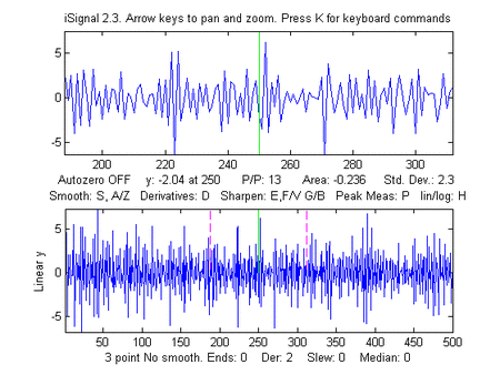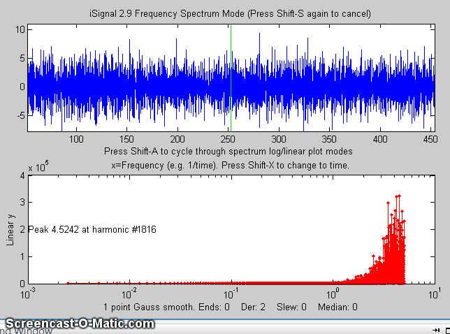This is the tool to use when you want to explore and clean up your signals and to try smoothing, differentiation, and peak sharpening. It measures things like peak-to-peak signal amplitude, standard deviation, frequency spectra, and the area under the curve of selected portions of your signal. It's also good for measuring peak positions, heights, areas (either one peak at a time or automatically) and for determining how smoothing, differentiation, and peak sharpening effect the signal and its frequency spectrum. It can also pre-process signals to re-sample them by interpolation, and reduce or remove artifacts such as spikes (with the median filter) and steps (with a rate-limiting filter).	Interactive smoothing and differentiation Frequency spectrum mode
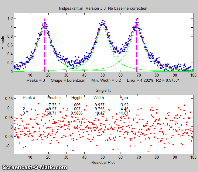
Peak Fitters  Peak fitting programs for time-series signals, which use a non-linear optimization algorithm to decompose a complex overlapping-peak signal into its component parts. The objective is to determine whether your signal can be represented as the sum of fundamental underlying peaks shapes. Accepts signals of any length, including those with non-integer and non-uniform x-values. Fits groups of peaks of many different shapes). There two different versions: (1) peakfit.m, a command line version, for Matlab and Octave, that fits a predetermined number of peaks, and findpeaksb.m and related functions that uses findpeaks.m to locate peaks as input for the peakfit.m function. If you have large sets of similar data that you need to fit automatically, you can put peakfit.m into a loop. This function is updated often, mostly to add new peak shape functions suggested by users, and it was elected the Matlab File Exchange "Pick of the Week" in 2016.   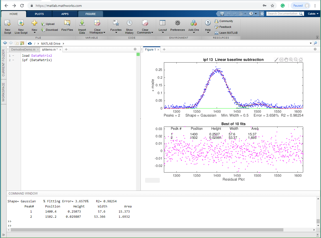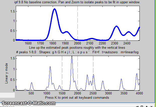(2) Interactive Peak Fitter, ipf.m, a keypress-operated interactive version, for Matlab (also available in an Octave version) that allows you to pan and zoom through the signal to pick the groups of peaks to fit. Does not work in Octave. There is an animated demonstration. Using ipf.m in Matlab, you can press a single keystroke to instantly adjust the data range, change the peak shape, number of peaks, baseline mode, or to re-calculate the fit with different start or with a bootstrap subset of the data. Super quick and easy. The difference between them is that peakfit.m is completely controlled by command-line input arguments and returns its information via command-line output arguments; ipf.m allows interactive control via keypress commands. Otherwise they have similar curve-fitting capabilities. You can also download a ZIP file containing peakfit.m, DemoPeakFit.m, ipf.m, Demoipf.m, some sample data for testing, and a test script (testpeakfit.m) that runs all the examples sequentially to test for proper operation.  These tools are the ones to use when (a) you need to measure the peak positions, amplitudes, widths, and areas of the positive peaks in your signal, (b) the peaks are highly overlapped, (c) you want specific peaks in your signal quantified, and (d) your peaks are approximately Gaussian, Lorentzian, Pearson, Logistic, or exponentially-  broadened Gaussian. You can use the interactive ifp.m function to determine the ideal input arguments for the peakfit.m and command-line function. Note: iterative non-linear curve fitting based on peakfit.m can also performed by the latest versions of iPeak and iSignal, both described above. For some demos comparing (older version of) peakfit.m and  iPeak.m, download idemos.zip.
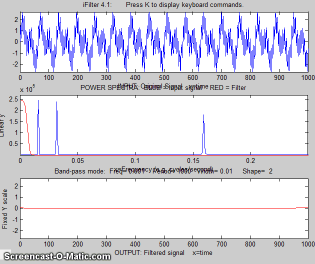
iFilter: Interactive Fourier Filter iFilter for Matlab, or ifilteroctave for Octave, is an interactive Fourier filter function for time-series signals that allows you to adjust the filter parameters continuously while observing the effect on your signal dynamically. Using keystrokes, you can create lowpass, highpass, bandpass, and band-reject (notch), comb pass, and comb reject filters with variable, frequency, width, and cut-off rate. The x-axis is labeled for time-based signals, where the independent variable is time in seconds, but the program can be used with any frequency axis (e.g. spacial frequency, etc).  Click here to view or download iFilter.m  You can also download it from the Matlab File Exchange. Version 4.1, December, 2014. Octave version December 2021. Press K to see the keystroke commands for that version. This is the tool to use when you want to explore the frequency components of your signals and to design a custom filter that will optimize your signals.
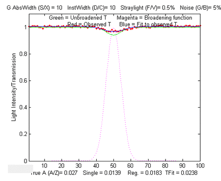
Hyperlinear quantitative absorption spectroscopy Matlab implementation of a computational method for quantitative analysis by multiwavelength absorption spectroscopy, called the transmission-fitting or "TFit" method, based on measuring the underlying absorbance by fitting a model of the instrumentally-broadened transmission spectrum to the observed transmission data, rather than by direct calculation of absorbance as simply log10(Izero/I).  Advantages of the TFit method compared to conventional methods are: (a) wider dynamic range; (b) greatly improved calibration linearity; (c) ability to operate under conditions that are optimized for signal-to-noise ratio ratio rather than for optical ideality. With a linear response, absorbance can be converted to concentration simply by multiplying by a constant factor. Just like the multilinear regression (classical least squares) methods conventionally used in absorption spectroscopy, the Tfit method (a) requires an accurate reference spectrum of each analyte, (b) utilizes multiwavelength data such as would be acquired on diode-array, Fourier transform, or automated scanning spectrometers, and (c) applies both to single-component and multi-component mixture analysis. tfit.m is a command-line demo function for Matlab or Octave. TFitDemo.m is an interactive demo m-file that works in recent versions of Matlab. Version 2.1, November 2011.
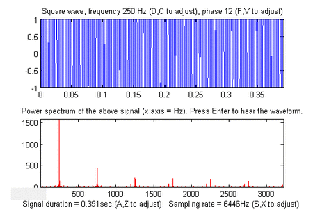
iPower: Interactive Power Spectrum Demo Matlab keyboard-controlled interactive power spectrum demonstrator, useful for teaching and learning about the power spectra of different types of signals and the effect of signal duration and sampling rate. Single keystrokes allow you to select the type of signal (12 different preset signals included), the total duration of the signal, the sampling rate, and the global variables f1 and f2 which are used in different ways in the different signals. If you know some basic Matlab programming, you can even add your own custom signal functions to this program. When the Enter key is pressed, the signal (y) is sent to the Windows WAVE audio device. Press K to see a list of all the keyboard commands. Click here to view or download.  You can also download it from the Matlab File Exchange. Version 2, October 2011
Diffraction Grating Demos A set of keyboard-controlled interactive demonstration modules, written as self-contained Matlab functions, that are useful for learning and teaching the principles of diffraction gratings. Shows a working cross section of the geometry of a diffraction grating (a common illustration in textbooks of optics, spectroscopy, and analytical chemistry). Single keystrokes allow you to control such variables as the angle of incidence, grating ruling density, wavelength, and diffraction order. One module shows how the operation of a diffraction grating emerges naturally just by adding up a bunch of sine waves, without any higher math at all.  Press K to see a list of all the keyboard commands. Tested in Matlab version 7.8 (R2009a). Click here to download ZIP file.  You can also download it from the Matlab File Exchange. Version 2, November 2011. There is also a set of spreadsheets in Excel (.xls) and OpenOffice (.ods) format that illustrate grating operation in an interactive way, with sliders and number wheels to change parameters.

(a) Make sure you don't click on the "Show Plot Tools" button in the toolbar above the figure; that will disable normal program functioning. If you do; close the Figure window and start again.

(b) To facilitate transfer of settings from one of these functions to another or to a command-line version,all these functions use the W key to print out the syntax of other related functions, with the pan and zoom settings and other numerical input arguments specified, ready for you to Copy, Paste and edit into your own scripts or back into the command window. For example, you can convert an iSignal.m operation onto a command-line ProcessSignal.m call, or a curve fit in ipf.m into the command-line peakfit.m function, or a peak finding operation from ipeak.m into the command-line findpeaksG.m or findpeaksb.m or findpeaksb3.m functions. This provides a way to deal with signals that require different signal processing in different regions of their x-axis ranges, by allowing you to create a series of command-line functions for each local region that, when executed in sequence, quickly process each segment of the signal appropriately. 

(c) Recent versions of these three programs use the Shift-Ctrl-S, Shift-Ctrl-F, and Shift-Ctrl-P keys to transfer the current signal between iSignal.m, ipf.m, and iPeak.m

2. Live Script functions.

A. Live script for smoothing

The script has several interactive controls. The two sliders in lines 9 and 10 allow you to select which portion of the data range to process, from 0% to 100% of the total range of the data file. The SmoothType drop-down menu in line 13 selects the smoothing algorithm; each has one or more controls specific to that type in lines 16 to 30. The first choice is the recursive sliding average (fastsmooth.m) algorithm explained above. The smooth width and number of passes are controlled by the sliders in lines 16 and 17. Each The other controls are explained in the accompanying comment lines (in green). Fourier filtering, Savitsky-Golay and wavelet denoising are topics that will be explained in other sections. The PlotBeforeAndAfter checkbox in line 3 gives you the option of plotting the original signal (in black) along with the processed signal (in red). The FrequencySpectra checkbox in line 4 allows you to show the frequency spectrum of the original and/or processed signals (see HarmonicAnalysis.html). Note: to view the graphic plots to the right of the code, as shown above, right-click on the empty space on the right and select "Disable synchronous scrolling".

B. Live script for self-deconvolution. 

DeconvoluteData.mlx can perform Fourier self-deconvolution on you own data stored in disk. Clicking the Open data file button in line 1 opens a file browser, allowing you to navigate to your data file in .csv or .xlsx format. (The script assumes that your x,y data are in the first two columns; you can change that in lines 13 and 14). In the case shown here, the data file is a portion of the IR spectrum of Heptene, 'HepteneTestData.csv', shown as the 'file' variable in the workspace. The The startpc and endpc sliders in lines 9 and 10 allow you to select which portion of the data range to process, from 0% to 100% of the total range of the data file.

The PeakShape drop-down menu in line 17 selects the convolution function shape (in this case, a Gaussian-Lorentzian blend) and the PCGaussian slider in the next line allows selection of the percent Gaussian of that shape. The dw slider in line 21 controls the deconvolution half-width, the DA slider in line 23 controls the percent denominator addition.  Smoothing, by Fourier filtering, is controlled by the FrequencyCutoff and CutOffRate in lines 25 and 27. All variables are accessible in the Matlab workspace; the final signal is 'syDA'.

Click the FrequencySpectra check box in line 4 to view the frequency spectra. Click the PlotAllSteps check box in line 5 to view all the steps leading up the the final result. To view the figures to the right as shown below, right-click on the right-hand panel and select "Disable synchronous scrolling".

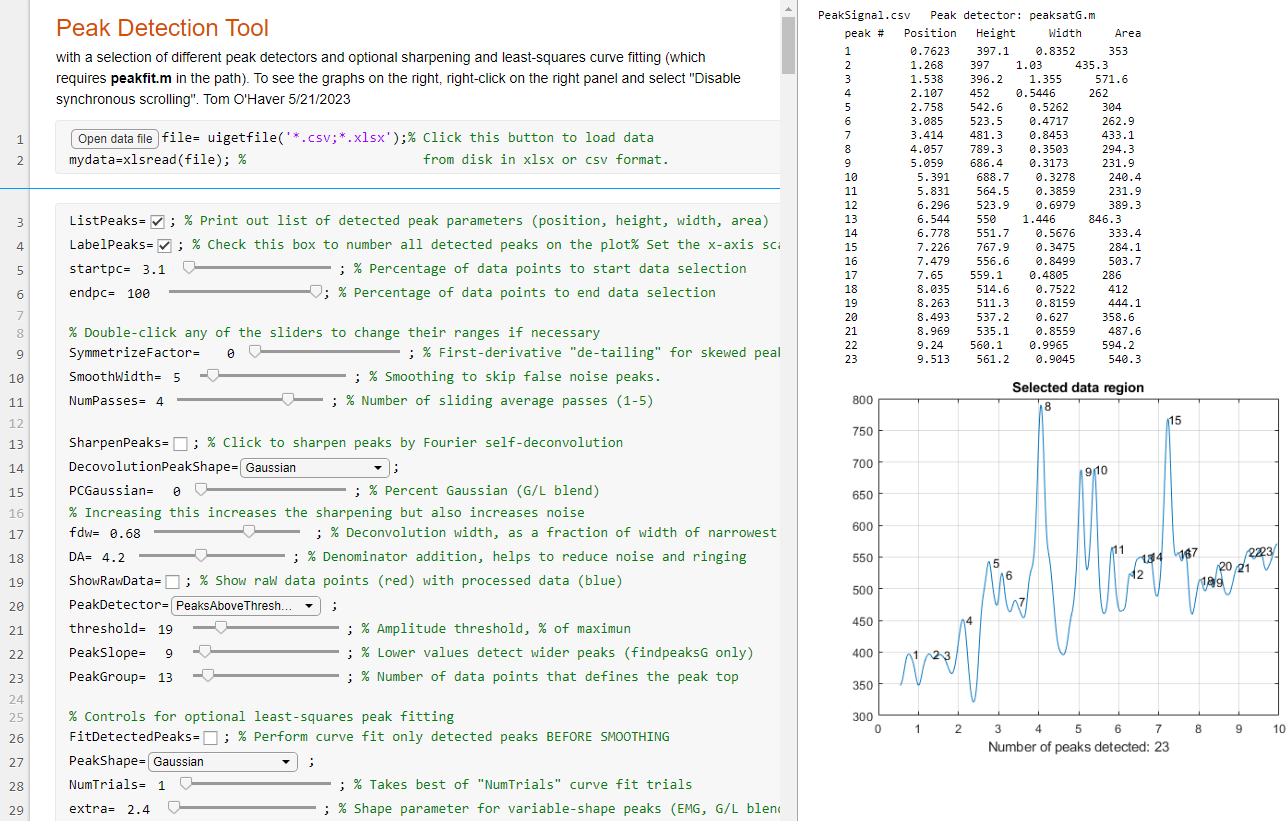
C. Peak detection tool

Clicking the OpenDataFile button in line 1 opens up a file browser, allowing you to navigate to your data file (in .csv or .xlsx format). The startpc and endpc sliders in lines 5 and 6 allow you to set the start and end of the region to focus on (expressed as a percentage of the total data length). You can set controls to smooth the data (lines 10 and 11) or to "de-tail" or symmetrize the peaks (line 9). You can choose a peak detector using the PeakDetector drop-down menu in line 20. The ListPeaks and LabelPeaks check boxes in lines 3 and 4 allow you to number the peaks on the graph and/or to display a list of peak parameters of the detected peaks. You can optionally try to sharpen the peaks, to enable detection of weak side peak or shoulders, by clicking the SharpenPeaks check box in line 13. Click the "Show raw data" check box to plot the raw data as red dots along with the processed (smoothed, sharpened, or symmetrized data). Smoothing, symmetrization, and sharpening all use area-preserving algorithms.

You can also apply iterative least-square curve fitting, by clicking the FitDetectedPeaks check box on line 26 and selecting the desired fitting function shape from the PeakShape drop-down menu on line 27. Here is an example. The position and width of the peaks estimated by the peak detectors is used as the first-guess starting point for the iterative fit; therefore only detected peaks will be included in the fit. This function requires that peakfit.m be in the Matlab path. (Normally, curve fitting is applied only to the unsmoothed data; however, if peak sharpening or symmetrization is applied (line 9 or 13), it uses the processed data).

The function of each of the controls is described in the associated comment lines. For examples of its application to several different kinds of peak data, see the PDF file PeakDetector.pdf, which references a set of .csv data files which as also downloadable from the same address.

(To see the graphs on the right as above, right-click on the right panel and select "Disable synchronous scrolling").

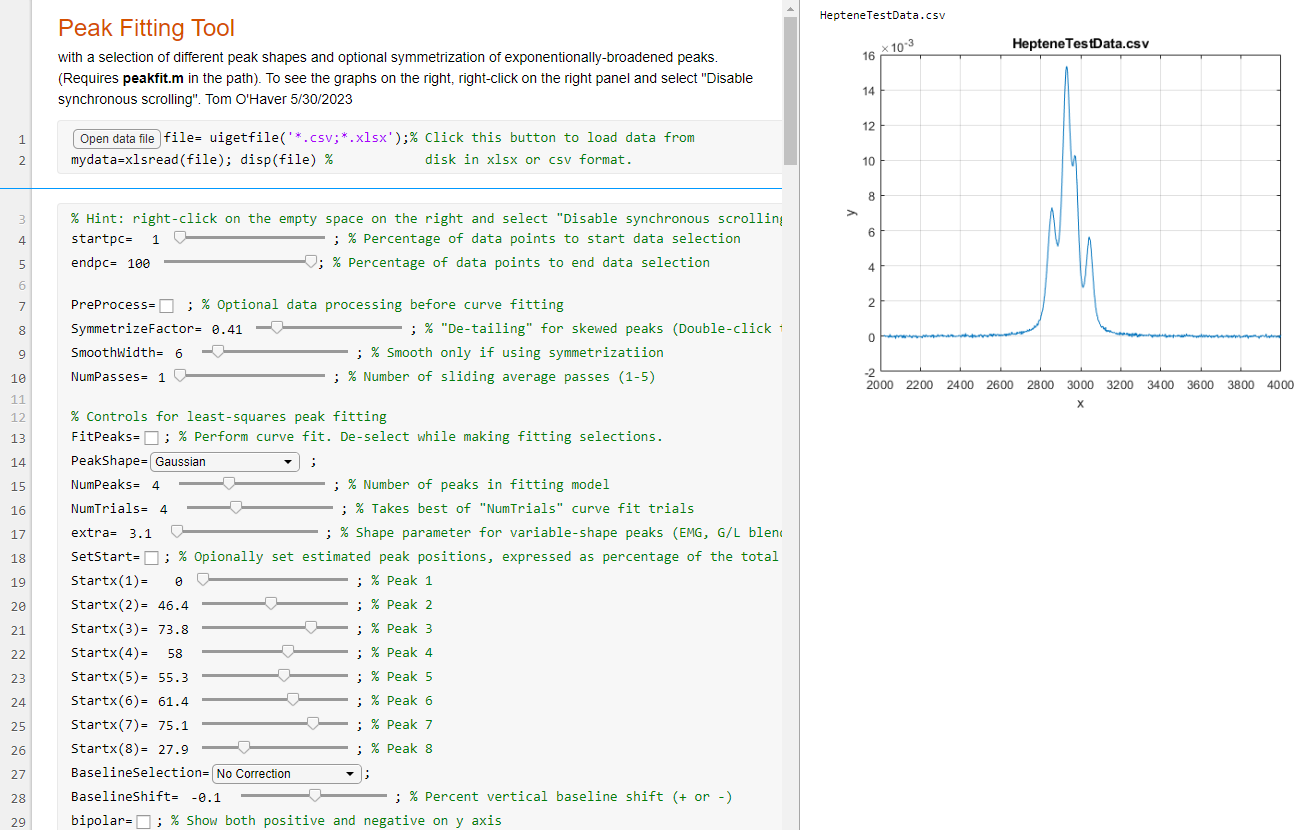
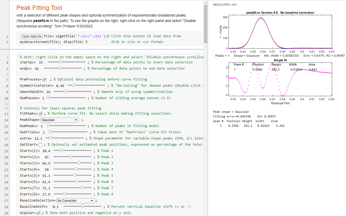
D. Peak Fitter tool

Like the other Live Scripts described above, PeakFittingTool.mlx has a file browser button in line 1 and a pair of sliders in lines 4 and 5 for setting the desired segment to work on. But before opening a file, it's a good idea to temporarily de-select the "FitPeaks" check-box in line 14, then when you have set all the other controls, click it back on. That way you will avoid waiting for unnecessary curve fit operations until the appropriate settings are complete. (Sometimes curve fitting operations can be slow and can take several seconds in difficult cases). With FitPeaks switched off, the program simply displays a plot of the selected data file.

Adjust the startpc and endpc sliders in lines 4 and 5 to isolate groups of closely-spaced peaks that can be fit together. Try to spread them out as evenly as possible, as shown in the figure above. (If all the peaks are well separated and do not overlap, you may be between off using the Peak Detector Tool (Peakdetector.mlx), which also has a peak fitting function).

The "PreProcess" check box (line 7) allows for some optional preliminary pre-processing. The SymmetrizeFactor slider preforms "symmetrization" or "de-tailing" for peaks that are skewed by exponential broadening, by means of the first-derivative addition. Increase the value of SymmetrizeFactor until the peak is as narrow as possible without the trailing edge falling below the baseline. The SmoothWidth and NumPasses sliders (lines 9 and 10) permit sliding average smoothing on the signal, which is useful for cases where high-frequency noise obscures the peaks. The "VerticalShift" slider (line 11) allows for positive and negative shift in the baseline position, to compensate for baseline offset.

The PeakShape drop-down menu allows you to select the peak shape of the fitting model. NumPeaks sets the number of peaks in the model. NumTrials, restarts the fitting process "NumTrials" times with slightly different start values and selects the best one (with lowest fitting error). NumTrials can be any positive integer. In many cases, NumTrials=1 will be sufficient, but if that does not give consistent results, increase it until the result are stable. The extra slider is used to fine-tune the certain peak shapes, e.g., the Pearson, exponentially-broadened Gaussian, and Gaussian/Lorentzian blend. Adjust this to minimize the fitting error.

After all of these setting have been made, then you can activate the FitPeaks check-box, a fit will be performed, and the resulting peak table displayed in the right-hand panel, as in the graphic above. Thereafter, any changes in the setting will cause an immediate recalculation of the curve fit.

In difficult cases, better results can be obtained if you specify the estimated positions of the peaks, especially if the peaks are very irregularly spaced or if some peaks appear only as shoulders or bulges rather than as distinct peaks. Select the SetStart check box and adjust the sliders to the predicted relative peak positions, for each peak in the model in lines 19 to 26. The length of these sliders represents the x-axis range displayed in the figure.

If the baseline for the group of peaks is offset from zero, you can correct that by using the BaselineShift slider in line 28. If the baseline for the group of peaks is tilted or curved, you can use the BaselineSelection menu in line 27 to choose a baseline correction that attempts to estimate the baseline from the edges of the signal range.

The Bipolar check box (line 29) controls whether to display both positive and negative signal values in the graphic or only positive values.

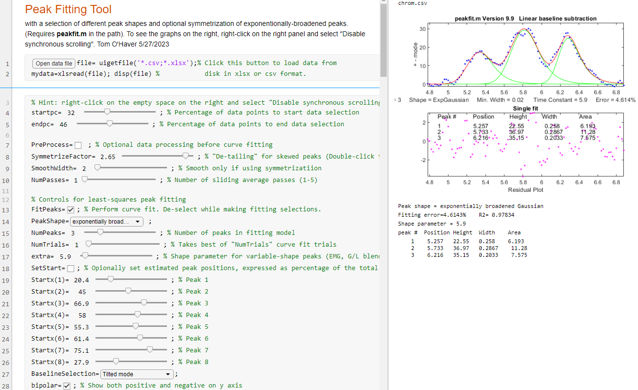
Another example of Peak Fitting Tool shows it fitting a group of weak peaks in narrow section of a much larger signal (chrom.csv), in this case using the exponentially broadened Gaussian shape and the "Tilted mode" baseline correction (line 27).   

Additional shapes may easily be added to the PeakShape menu by selecting other shapes form the list of predefined shapes and their corresponding number on https://terpconnect.umd.edu/~toh/spectrum/InteractivePeakFitter.htm, adding that name and number to the others in the switch/case statement in lines 52-73, then adding that new shape to the drop-down menu on line 15. Just follow that pattern of the shapes already there.

In fitting asymmetrical peaks what have an exponential skew, you can either try to remove the asymmetry by using the SymmetrizeFactor slider (example) followed by fitting a symmetrical peak shape or by selecting an exponentially broadened peak shape (example); both approaches can yield similar results as in these examples, but the former method is often faster.

Verbatim Unsolicited Comments from Users of my Matlab codes

"Your program iPeak is like falling out of a tree and landing in a soft couch complete with a book and a good reading light!" 

"Your peakfit script is simply phenomenal!"

"Fantastic Matlab code"

"Very beautiful script!"

"...awesome functions!"

"... perfect documentation."

"This is great, exactly what I was looking for."

"...after days of trying and failing...I stumbled upon your site and was able to solve my problem in half an hour."

"... surely the way into heaven is to post excellent software online for others to use to do science."

"This makes me so incredibly happy!"

"your matlab scripts are really beautiful...."

"...a fantastic tool...extremely efficient."

"...exactly the tool I was searching for after struggling with my data for days."

"I used the peakfit.m program to analyze some Raman data and found it to be incredibly useful."

"... great software package."

"...awesome MATLAB peakfiting script..."

"...[ipf.m] is a really useful bit of code"

"...your wonderful [peak fitter] program. I use it on a regular basis...."

"peakfit is amazing!'

"I have been using iPeak ... (awesome program!!)."

"Interactive Peak Fitter [ipf.m]...worked very well. In a word, it's perfect！"

"... your functions are all incredibly helpful...." 

"...iSignal 3...is a great tool!!"

"Your code is quite amazing."

"[peakfit.m] is really well designed and allows numerous fit...."

"Great function...I've used this for years..."

"...love your iPeak program!"

"I've just download your very nice PeakFitter. It's WONDERFUL!"

"You have great detailed instructions!"

"your excel sheet for spectral deconvolution ... worked beautifully."

"...how awesome your peakfitter is!"

"...you can't imagine how MUCH we'll use this."

"...thank you for taking the time to create these incredible tools."

"This [peakfit.m] function is so powerful and simple to use."

"I am really impressed with the extensive package you have put together - I am finding it very helpful.

"...your scripts findpeaks.m and ipeaks.m ... [are] super useful"

"...great documentation...outstanding functions."

" ...the scripts that you developed which are a very useful help for a lot of people in science research."

"I got some really good results using Ipeak.

"This program [Peak Fitter] is perfect."

"I find these routines and the information on your website immensely valuable."

"I recently found your website and I'm really impressed, great work! "

" Your spreadsheets got me rolling quickly!"

"...your tools...are very well made."

"I have been using your "findpeaks" routine (matlab version) and it is working superbly."

"Your peak picking algorithm is very helpful to me."

"As far as I am concerned your code is perfect..."

"Your peakfit function is very powerful. I had test many data with success."

"I'm impressed at the convenience of your Peak Fitter and Interactive Peak Fitter programs."

"I found your Peak Fitter program to be incredibly useful for some work I am doing...."

"I found your Matlab functions for peak detection very useful for my research. Thanks for making this resource available, it's been of great help to me". 

"Best fitter available for Matlab, thanks for this wonderful work."

"...hank you for the great work you done with the peak finding methods for Matlab. It is really great."

"I've been using ipeak over the past few weeks and this is a wonderful tool."

"These are very good script(s)....The scripts are very useful to help to solve my problem...."

"[It's] exactly what I needed....The result looks really great!"

"...your interactive peak fitter Matlab tool...it's a wonderfully powerful and easy to use program.  I have been recommending it to everyone who asks for peak fitting programs".  

"Great code....Wonderfully documented!

"I am using your peakfitter in Matlab and love it....worked like a charm" 

"I've been having great success with ipf and peakfit..."

"...it really is a fine manual - your pdf document on curve fitting." 

"Your Interactive Peak Fitter ... is very helpful."

"Your peak finding and fitting scripts ... turned out handy in analyzing my research data."

"I found your peakfit.m program and it is great - thank you very much for sharing it!"

"...the codes for finding peaks and mathematical fits to noisy data...were very helpful for my experimental work."

"I appreciate all the work that must have gone into the PeakFit matlab coding. I've been using it ... and it is becoming extremely useful."

",,,your Matlab function findpeaks()...is quite literally EXACTLY what I was looking for and far better than I could have hoped."

"...MATLAB code for scientists! It's such a great resource to have.... I really appreciate your efforts."

"Thank you for making available your absolutely superb Peakfinder software. It is a snap to use...."

"...thanks for the great tool! Saved me a lot of work."

"...iPeak ... is very useful."

"...your scripts are wonderful."

"...really nice tutorial and Matlab functions that are extremely useful in many fields of research."

"I used your peakfit MATLAB file in a paper. I found it VERY useful ."

"I have been impressed by your MATLAB codes."

"Wow! ... this is exactly what I needed."

"You programs work very well and are very helpful to me. "

"...very convenient and well-written..."

"...your interactive peak fitter code for Matlab...has been very useful!"

Copyright (c) 2014, 2021 Thomas C. O'Haver
 
Permission is hereby granted, free of charge, to any person obtaining a copy of this software and associated documentation files (the "Software"), to deal in the Software without restriction, including without limitation the rights to use, copy, modify, merge, publish, distribute, sub-license, and/or sell copies of the Software, and to permit persons to whom the Software is furnished to do so, subject to the following conditions:

The above copyright notice and this permission notice shall be included in all copies or substantial portions of the Software.

THE SOFTWARE IS PROVIDED "AS IS", WITHOUT WARRANTY OF ANY KIND, EXPRESS OR IMPLIED, INCLUDING BUT NOT LIMITED TO THE WARRANTIES OF MERCHANTABILITY, FITNESS FOR A PARTICULAR PURPOSE AND NONINFRINGEMENT. IN NO EVENT SHALL THE AUTHORS OR COPYRIGHT HOLDERS BE LIABLE FOR ANY CLAIM, DAMAGES OR OTHER LIABILITY, WHETHER IN AN ACTION OF CONTRACT, TORT OR OTHERWISE, ARISING FROM, OUT OF OR IN CONNECTION WITH THE SOFTWARE OR THE USE OR OTHER DEALINGS IN THE SOFTWARE.