(a) much wider dynamic range (i.e., the concentration range over which one calibration curve can be expected to give good results) ,
(b) greatly improved calibration linearity ("hyperlinearily"), which reduces the labor and cost of preparing and running large numbers of standard solutions and safely disposing of them afterwards, and
(c) the ability to operate under conditions that are optimized for signal-to-noise ratio rather than for Beer's Law ideality, that is, small spectrometers with shorter focal length, lower dispersion and larger slit widths to increase light throughput and reduce the effect of photon and detector noise (assuming, of course, that the detector is not saturated or overloaded).
Just like the multilinear
regression (classical least squares) methods conventionally
used in absorption spectroscopy, the Tfit method
(a) requires an accurate reference spectrum of each analyte,
(b) utilizes multiwavelength data such as would be acquired on diode-array, Fourier transform, or automated scanning spectrometers,
(c) applies both to single-component and multicomponent mixture analysis, and
(d) requires that the absorbances of the components vary with wavelength, and, for multi-component analysis, that the absorption spectra of the components be sufficiently different. Black or grey absorbers do not work with this method.
The disadvantages of the Tfit method are:
(a) it makes the computer work harder than the multilinear regression methods (but, on a typical personal computer, calculations take only a fraction of a second, even for the analysis of a mixture of several components);
(b) it requires knowledge of the instrument function, i.e., the slit function or the resolution function of an optical spectrometer (however, this is a fixed characteristic of the instrument and can be measured beforehand by scanning the spectrum of a narrow atomic line source such as a hollow cathode lamp). It changes only if you change the slit width of the spectrometer;
(c) it is an iterative method that can under unfavorable circumstances converge on an incorrect local optimum, but this is handled by proper selection of the starting values calculated by the traditional log (Io/I) method), and
(d) It won't work for gray-colored substances whose absorption spectra do not vary over the spectral region measured.
Click here to download an interactive
self-contained demo m-file that works in recent versions of
Matlab. You can also download a ZIP file
"TFit.zip" that contains both the interactive version for
Matlab and a command-line version for Octave.
You can also download it from the Matlab
File Exchange. There is also a spreadsheet
version.
The following sections give the background
of the method and a description of the main function and demonstration
programs and spreadsheet templates:

 The
graphic here shows a simplified layout of a typical optical
absorption spectroscopy measurement. Light of a specific
wavelength range passes through an absorbing sample and is measured
by a photodetector. The intensity I of light passing through the sample is
given (in Matlab notation) by the Beer-Lambert
Law:
The
graphic here shows a simplified layout of a typical optical
absorption spectroscopy measurement. Light of a specific
wavelength range passes through an absorbing sample and is measured
by a photodetector. The intensity I of light passing through the sample is
given (in Matlab notation) by the Beer-Lambert
Law:
I = Io.*10^-(alpha*L*c)
where "Io"
(pronounced "eye-zero") is the intensity of the light incident on
the sample, "alpha" is the absorption coefficient of the absorber,
"L" is the
distance that the light travels through the material (the path
length), and "c"' is the concentration of absorber in the sample.
The variables I, Io,
and alpha are all functions of wavelength; L and c are scalar.
In conventional applications, measured values of I and Io are used to compute the quantity called "absorbance", defined as
A = log10(Io/I)
Absorbance is defined in this way so that, when you combine this
definition with the Beer-Lambert law, you get:
A = alpha*L*c
So, absorbance is proportional to concentration, ideally, which simplifies analytical calibration. However, any real spectrometer has a finite spectral resolution, meaning that the light beam passing through the sample is not truly monochromatic, with the result that an intensity reading at one wavelength setting is actually an average over a small spectral interval. More exactly, what is actually measured is a convolution of the true spectrum of the absorber and the instrument function, the instrument's response as a function of wavelength of the light. Ideally the instrument function is infinitely narrow (a "delta" function), but practical spectrometers have a non-zero slit width, the width of the adjustable aperture in the diagram above, which passes a small spectral interval of wavelengths of light from the dispersing element (prism) onto the sample and detector. If the absorption coefficient "alpha" varies over that spectral interval, then the calculated absorbance will no longer be linearly proportional to concentration (this is called the "polychromicity" error). The effect is most noticeable at high absorbances. In practice, many instruments will become non-linear starting at an absorbance of 2 (~1% Transmission). As the absorbance increases, the effect of unabsorbed stray light and instrument noise also becomes more significant.
The theoretical best signal-to-noise ratio and absorbance precision for a photon-noise limited optical absorption instrument can be shown to be close to an absorbance close to 1.0 (see Is there an optimum absorbance for best signal-to-noise ratio?). The range of absorbances below 1.0 is easily accessible down to at least 0.001, but the range above 1.0 is limited. Even an absorbance of 10 is unreachable on most instruments and the direct measurement of an absorbance of 100 is unthinkable, as it implies the measurement of light attenuation of 100 powers of ten - no real measurement system has a dynamic range even close to that. In practice, it is difficult to achieve an dynamic range even as high as 5 or 6 absorbance, so that much of the theoretically optimum absorbance range is actually unusable. (c.f. http://en.wikipedia.org/wiki/Absorbance). So, in conventional practice, greater sample dilutions and shorter path lengths are required to force the absorbance range to lower values, even if this means poorer signal-to-noise ratio and measurement precision at the low end.
It
is true that the non-linearity caused by polychromicity can be
reduced by operating the instrument at the highest resolution
setting (reducing the instrumental slit width). However, this has
a serious undesired side effect: in dispersive
instruments, reducing the slit width to increase the
spectral resolution degrades the signal-to-noise substantially. It
also reduces the number of atoms or molecules that are actually
measured. Here's why: UV/visible absorption spectroscopy is based
on the the absorption of photons of light by molecules or atoms
resulting from transitions between electronic energy states. It's
well known that the absorption peaks of molecules are more-or-less
wide bands, not monochromatic lines, because the molecules are
undergoing vibrational and rotational transitions as well and are
also under the perturbing influence of their environment. This is
the case also in atomic
absorption spectroscopy: the absorption "lines" of
gas-phase free atoms, although much narrower that molecular bands,
have a finite non-zero width, mainly due to their velocity
(temperature or Doppler broadening) and collisions with the matrix
gas (pressure broadening). A macroscopic collection of molecules
or atoms, therefore, presents to the incident light beam a distribution
of energy states and absorption wavelengths. Absorption
results from the collective interaction of many individual atoms
or molecules with individual photons. A purely monochromatic
incident light beam would have photons all of the same
energy, ideally corresponding to the average energy distribution
of the collection of atoms or molecules being measured. But many -
actually most - of the atoms or molecules would have a energy
greater or less than the average and would thus not be
measured. If the bandwidth of the incident beam is
increased, more of those non-average atoms or molecules would be
available to be measured, but then the simple calculation of
absorbance as log10(Io/I) is no longer valid and would result in a
non-linear response to concentration.
Numerical simulations
show that the optimum signal-to-noise ratio is typically achieved
when the spectral resolution of
the instrument approximately matches the width of the analyte
absorption, but then using the conventional log10(Io/I)
absorbance would result in very substantial non-linearity over
most of the absorbance range because of the polychromicity error. This
non-linearity has its origin in the spectral domain
(intensity vs wavelength), not in the calibration domain
(absorbance vs concentration). Therefore it should be no surprise
that curve fitting in the calibration domain, for example fitting
the calibration data with a quadratic or cubic fit, would not be
the best solution, because there is no theory that says that the
deviations from linearity would be expected to be exactly
quadratic or cubic. A more theory-based approach would be to
perform the curve fitting in the spectral domain where
the source of the non-linearity arises. 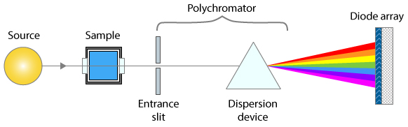 This is possible with
modern absorption spectrophotometers that use array
detectors, which have many tiny detector elements that slice
up the spectrum of the transmitted beam into many small wavelength
segments, rather than detecting the sum of all those segments with
one big photo-tube detector, as older instruments do. An
instrument with an array detector typically uses a slightly
different optical arrangement, as shown by the simplified diagram
on the left, where the spectral resolution is determined by both
the entrance slit and the range of optical detector elements that
are summed to determine the transmitted intensity.
This is possible with
modern absorption spectrophotometers that use array
detectors, which have many tiny detector elements that slice
up the spectrum of the transmitted beam into many small wavelength
segments, rather than detecting the sum of all those segments with
one big photo-tube detector, as older instruments do. An
instrument with an array detector typically uses a slightly
different optical arrangement, as shown by the simplified diagram
on the left, where the spectral resolution is determined by both
the entrance slit and the range of optical detector elements that
are summed to determine the transmitted intensity.
The TFit method sidesteps the above problems by calculating the
absorbance in a completely different way: it starts with the
reference spectra (an accurate absorption spectrum for each
analyte, also required by the multilinear regression methods),
normalizes them to unit height, multiplies each by an adjustable
coefficient - initially equal to the conventional log10(Io/I)
absorbance - adds them up, computes the antilog, and convolutes it
with the previously-measured slit function. The result,
representing the instrumentally broadened transmission spectrum,
is compared to the observed transmission spectrum. The
coefficients (one for each unknown component in the mixture) are
adjusted by the program until the computed transmission model is a
least-squares best fit to the observed transmission spectrum. The
best-fit coefficients are then equal to the absorbances determined
under ideal optical conditions. Provision is also made to
compensate for unabsorbed stray light and changes in background
intensity (background absorption). These calculations are
performed by the function fitM, which is
used as a fitting function for Matlab's iterative non-linear
fitting function fminsearch. The
TFit method gives measurements of absorbance that are much closer
to the "true" peak absorbance that would have been measured in the
absence of stray light and polychromatic light errors. More
important, it allows linear and wide dynamic range measurements to
be made even if the slit width of the instrument is increased to
optimize the signal-to-noise ratio.
From a historical perspective, by the time Pierre Bouguer
discovered what became to be known as the Beer-Lambert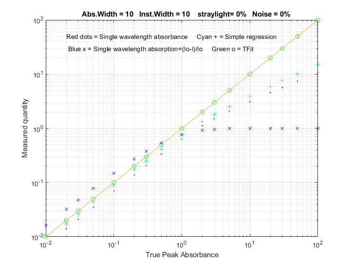 law in 1729, the logarithm was already well known,
having been introduced by John
Napier in 1614. So the additional mathematical work needed
to compute the absorbance, log(Io/I), rather than the
simpler relative absorption, (Io-I)/Io, was justified
because of the better linearity of absorbance with respect to
concentration and path length, and the calculation could easily be
performed simply by a slide-rule
type graduated scale. Certainly by today's standards, the
calculation of a logarithm is considered routine. In contrast, the
TFit method presented here is far more mathematically complex than
a logarithm and cannot be done without the aid of software
(minimally a spreadsheet) and some sort of computational
hardware, but it offers a further improvement in linearity
beyond that achieved by the logarithmic calculation of absorbance,
and it additionally allows the small slit width limitation to be
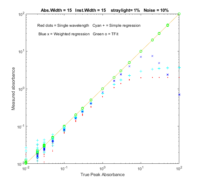
loosened. The figure on the right compares the analytical curve
linearity of simple relative absorption (blue x),
logarithmic absorbance (red dots), multilinear regression or CLS
method (cyan +) based on absorbance, and the TFit method (green
o). This plot was created by the Matlab/Octave script TFitCalCurveAbs.m.
law in 1729, the logarithm was already well known,
having been introduced by John
Napier in 1614. So the additional mathematical work needed
to compute the absorbance, log(Io/I), rather than the
simpler relative absorption, (Io-I)/Io, was justified
because of the better linearity of absorbance with respect to
concentration and path length, and the calculation could easily be
performed simply by a slide-rule
type graduated scale. Certainly by today's standards, the
calculation of a logarithm is considered routine. In contrast, the
TFit method presented here is far more mathematically complex than
a logarithm and cannot be done without the aid of software
(minimally a spreadsheet) and some sort of computational
hardware, but it offers a further improvement in linearity
beyond that achieved by the logarithmic calculation of absorbance,
and it additionally allows the small slit width limitation to be
loosened. The figure on the right compares the analytical curve
linearity of simple relative absorption (blue x),
logarithmic absorbance (red dots), multilinear regression or CLS
method (cyan +) based on absorbance, and the TFit method (green
o). This plot was created by the Matlab/Octave script TFitCalCurveAbs.m.
Bottom line: The TFit method is based on the
Beer-Lambert Law; it simply calculates the absorbance
in a different way that does not require the assumption that
stray light and polychromatic radiation effects are zero. Because
it allows larger slit widths and shorter focal lengths to be used,
it yields greater signal-to-noise ratios while still achieving a
much wider linear dynamic range than previous methods, thus
requiring fewer standards to properly define the calibration curve
and avoiding the need for non-linear calibration models. Keep in
mind that the log(Io/I) absorbance calculation is a 165-year-old
simplification that was driven by the need for
mathematical convenience, and by the mathematical skills of
the college students to whom this subject is typically first
presented, not by the desire to optimize detection
sensitivity and signal-to-noise ratio. It dates from the time
before electronics and computers, when the only computational
tools were pen and paper and slide rules, and when a method such
as described here would have been unthinkable. That was then; this
is now. Tfit is the 21st
century way to do quantitative absorption spectrophotometry.
Note: The TFit method compensates for the non-linearity caused by unabsorbed stray light and the polychromatic light effect, but other potential sources of non-linearity remain, in particular chemical effects, such as photolysis, equilibrium shifts, temperature and pH effects, binding, dimerization, polymerization, molecular phototropism, fluorescence, etc. A well-designed quantitative analytical method is designed to minimize those effects.
The
Tfit method can also be implemented in an Excel or
Calc spreadsheet; it's a bit more
cumbersome that the Matlab/Octave implementation, but it
works. The shift-and-multiply method is used for the
convolution of the reference spectrum with the slit
function, and the "Solver" add-in for Excel and Calc
is used for the iterative fitting of the model to the
observed transmission spectrum. This external source,
https://www.wallstreetmojo.com/solver-in-excel/,
has a detailed graphical explanation of using the
Solver. It's very handy, but not essential, to have a
"macro" capability to automate the process (See http://peltiertech.com/Excel/SolverVBA.html#Solver2
for more info about setting up macros and solver on
your version of Excel).
TransmissionFittingTemplate.xls
(screen image)
is an empty template; all you have to do is to enter
the data in the cells marked by a gray background:
wavelength (Column A), observed absorbance of
the sample (Column B), the high-resolution
reference absorbance spectrum (Column D), the
stray light (A6) and the slit function used for
the observed
absorbance of the sample (M6-AC6).
(TransmissionFittingTemplateExample.xls
(screen
image) is
the same template with example data entered.
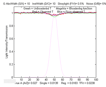
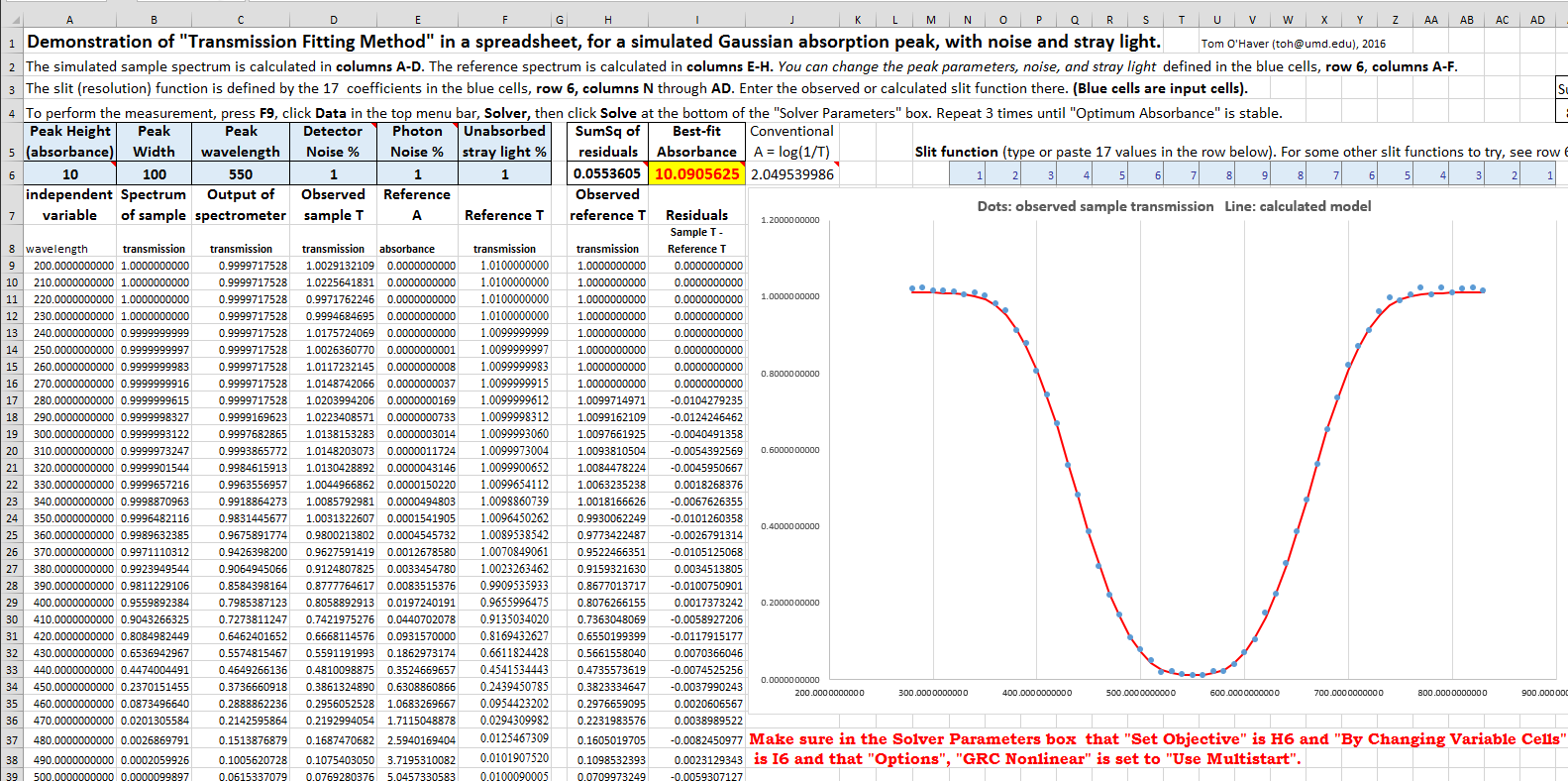
TransmissionFittingDemoGaussian.xls
(screen
image) is a demonstration with a simulated
Gaussian absorption peak
with variable peak position, width, and height, plus
added stray light, photon noise, and detector noise,
as viewed by a spectrometer with a triangular slit
function. You can vary all the parameters and compare
the best-fit absorbance to the true peak height and to
the conventional log(1/T) absorbance.
All of these spreadsheets include a macro, activated by pressing Ctrl-f,
that uses the Solver function to perform the iterative
least-squares calculation (see CaseStudies.html#Using_Macros).
But if you prefer not to use macros, you can do it
manually by clicking the Data tab, Solver,
Solve, and then OK.
TransmissionFittingCalibrationCurve.xls
(screen
image) is a demonstration spreadsheet that
includes another Excel macro
that constructs calibration curves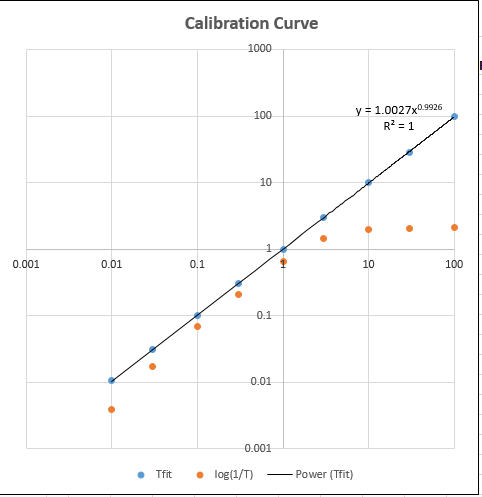 comparing the TFit and conventional log(1/T)
methods for a series of 9 standard
concentrations that you can specify.
To create a calibration curve, enter the
standard concentrations in AF10 - AF18 (or just
use the ones already
there, which cover
a 10,000-fold
concentration
range from 0.01 to 100), then press Ctrl-f
to run the macro. In this spreadsheet the macro does a lot more than in the
previous example:
it automatically goes through the
first row of the little table in
AF10 - AH18, extracts each
concentration value in turn,
places it in the
concentration cell A6, recalculates the
spreadsheet, takes the resulting
conventional absorbance (cell J6) and places
it as the first guess in cell I6, brings up
the Solver to compute the best-fit
absorbance for that peak height, places both
the conventional
absorbance and the
best-fit
absorbance in
the
table in
AF10 - AH18,
then goes to the next concentration and
repeats for each concentration value. Then it
constructs and
plots the log-log calibration curve (shown
on the right) for both the TFit method
(blue dots) and the
conventional (red
dots)
and computes the
trend-line equation and
the R2 value for the TFit
method, in the upper right
corner of graph. Each time
you press Ctrl-f it
repeats the whole
calibration curve with
another set of random
noise samples. (Note: you
can also use this
spreadsheet to compare the
precision and reproducibility
of the two methods by entering
the same concentration
9 times in AF10
- AF18.
The result should
ideally be a straight
flat line with
zero slope).
comparing the TFit and conventional log(1/T)
methods for a series of 9 standard
concentrations that you can specify.
To create a calibration curve, enter the
standard concentrations in AF10 - AF18 (or just
use the ones already
there, which cover
a 10,000-fold
concentration
range from 0.01 to 100), then press Ctrl-f
to run the macro. In this spreadsheet the macro does a lot more than in the
previous example:
it automatically goes through the
first row of the little table in
AF10 - AH18, extracts each
concentration value in turn,
places it in the
concentration cell A6, recalculates the
spreadsheet, takes the resulting
conventional absorbance (cell J6) and places
it as the first guess in cell I6, brings up
the Solver to compute the best-fit
absorbance for that peak height, places both
the conventional
absorbance and the
best-fit
absorbance in
the
table in
AF10 - AH18,
then goes to the next concentration and
repeats for each concentration value. Then it
constructs and
plots the log-log calibration curve (shown
on the right) for both the TFit method
(blue dots) and the
conventional (red
dots)
and computes the
trend-line equation and
the R2 value for the TFit
method, in the upper right
corner of graph. Each time
you press Ctrl-f it
repeats the whole
calibration curve with
another set of random
noise samples. (Note: you
can also use this
spreadsheet to compare the
precision and reproducibility
of the two methods by entering
the same concentration
9 times in AF10
- AF18.
The result should
ideally be a straight
flat line with
zero slope).
Typical use:
absorbance =
fminsearch(@(lambda)(fitM(lambda, yobsd, TrueSpectrum,
InstFun, straylight)), start);
where start is the first guess (or
guesses) of the absorbance(s) of the analyte(s); it's
convenient to use the conventional log10(Io/I) estimate of
absorbance for start. The other arguments
(described above) are passed on to FitM. In this example, fminsearch
returns the value of absorbance that would have been measured in
the absence of stray light and polychromatic light errors (which
is either a single value or a vector of absorbances, if it is a
multi-component analysis). The absorbance can then be converted
into concentration by any of the usual
calibration procedures (Beer's Law, external standards, standard
addition, etc.).
Here is a specific numerical example,
for a single-component measurement where the true
absorbance is 1.00, using only 4-point spectra for
illustrative simplicity (of course, array-detector systems would
acquire many more wavelengths than that, but the
principle is the same). In this particular case the instrument
width (InstFun) is twice the absorption width, the stray
light is constant at 0.01 (1%). The conventional single-wavelength
estimate of absorbance is too low: log10(1/.38696)=0.4123.
In contrast, the TFit method using fitM:
yobsd=[0.56529 0.38696 0.56529 0.73496]';
TrueSpectrum=[0.2 1 0.2 0.058824]';
InstFun=[1 0.5 0.0625 0.5]';
straylight=.01;
start=.4;
absorbance=fminsearch(@(lambda)(fitM(lambda,yobsd,...
TrueSpectrum,InstFun,straylight)),start)
absorbance=([weight weight].*[Background RefSpec])\where RefSpec is the matrix of reference spectra of all of the pure components. You can see that, in addition to the RefSpec and observed transmission spectrum (yobsd), the TFit method also requires a measurement of the Instrument function (spectral bandpass) and the stray light (which the linear regression methods assume to be zero), but these are characteristics of the spectrometer and need be done only once for a given spectrometer.
(-log10(yobsd).*weight)
Simple script that computes the statistics of the TFit method
compared to single- wavelength (SingleW), simple regression
(SimpleR), and weighted regression (WeightR) methods. Simulates
photon noise, unabsorbed stray light and random background
intensity shifts. Estimates the precision and accuracy of the four
methods by repeating the calculations 50 times with different
random noise samples. Computes the mean, relative percent standard
deviation, and relative percent deviation from true absorbance.
Parameters are easily changed in lines 19 - 26. Results are
displayed in the MATLAB command window.
In the sample output shown on the left, results for true
absorbances of 0.001 and 100 are computed, demonstrating that the
accuracy and the precision of the TFit method is superior to the
other methods over a 10,000-fold range.
This statistics function is included as a keypress command (Tab key) in TFitDemo.m.
    True A    SingleW   SimpleR   WeightR   TFit
MeanResult =
    0.0010    0.0004    0.0005    0.0006    0.0010
PercentRelativeStandardDeviation =
  1.0e+003 *
    0.0000    1.0318    1.4230    0.0152    0.0140
PercentAccuracy =
    0.0000  -60.1090  -45.1035  -38.6300    0.4898
MeanResult =
  100.0000    2.0038    3.7013   57.1530   99.9967
PercentRelativeStandardDeviation =
         0    0.2252    0.2318    0.0784    0.0682
PercentAccuracy =
         0  -97.9962  -96.2987  -42.8470   -0.0033
Function that compares the analytical curves for
single-wavelength, simple regression, weighted regression, and the
TFit method over any specified absorbance range (specified by the
vector "absorbancelist" in line 20). Simulates photon noise,
unabsorbed stray light and random background intensity shifts.
Plots a log-log scatter plot with each repeat measurement plotted
as a separate point (so you can see the scatter of points at low
absorbances). The parameters can be changed in lines 20 - 27.
In the sample result shown on the left, analytical curves for the
four methods are computed over a 10,000-fold range, up to a peak
absorbance of 100, demonstrating that the TFit method (shown by
the green circles) is much more nearly linear over the whole range
than the single-wavelength, simple regression, or weighted
regression methods.The wide linearity range of Tfit is
especially important in regulated laboratories where anything
but linear least-squares fits to the calibration curve are discouraged.
This calibration curve function is included as a keypress command
(M key) in TFitDemo.m.

Figure
No. 1 window: Click to enlarge

Figure
No. 2 window: Click to enlarge
TFit3Demo.m and
TFit3DemoOctave
use keystrokes to interactively control the simulation parameters.
Both versions use the same keystrokes.
KEYBOARD
COMMANDS
A1
A/Z
Increase/decrease true absorbance of comp 1
A2
S/X Increase/decrease true absorbance of comp 2
A3
D/C Increase/decrease true absorbance of comp 3
Sepn
F/V Increase/decrease spectral separation
InstWidth
G/B Increase/decrease width of instrument
function (spectral bandpass)
Noise
H/N Increase/decrease random noise level when
InstWidth = 1
Peak
shape Q
Toggles between Gaussian and Lorentzian
absorption peak shape
Table
Tab Print
table of results
K
Print this list of keyboard commands
Sample table of results (by pressing the Tab
key):
--------------------------------------------------------
True
Weighted
TFit
Absorbance
Regression method
Component 1 3
2.06
3.001
Component 2 0.1
0.4316
0.09829
Component 3 5
2.464
4.998
Created October 03, 2006. Revised January, 2022.
(c) Tom O'Haver
Professor Emeritus
Department of Chemistry and Biochemistry
The University of Maryland at College Park
toh@umd.edu
http://terpconnect.umd.edu/~toh/
This page is part of "A
Pragmatic Introduction to Signal Processing", created
and maintained by Prof.
Tom O'Haver , Department of Chemistry and Biochemistry, The
University of Maryland at College Park. Comments, suggestions and
questions should be directed to Prof. O'Haver at toh@umd.edu. Updated December 2021.