iSignal is a downloadable interactive
multipurpose signal processing Matlab function that includes smoothing, differentiation, peak sharpening
(resolution enhancement), Fourier
frequency spectrum, least-squares
peak fitting, and other useful functions on time-series
data. It is written as a single self-contained function. Using
simple keystrokes, you can adjust the signal processing parameters
continuously while observing the effect on your signal
dynamically. Click here to
download the ZIP file "iSignal8.zip" that also includes some
sample data for testing. You can also download iSignal from the Matlab
File Exchange. If you are using Octave instead of Matlab,
use the Octave
version, which uses different keys for pan and zoom. Press
the K key to list the keystroke commands.
Last few versions: Version 8.3, May 2020 add constant
denominator addition to deconvolution options, to reduce ringing and
noise (the "5" and "6" keys change the added constant). Version 8.2,
April 2020. Interactive convolution and deconvolution, "Shift V" key
to select from menu; "3" and "4" keys change the width by 10% and
"Shift-3" and "Shift-4" keys change by 1%. Version 7, June 2019. Symmetrize
exponentially broadened peaks peaks by weighted first
derivative addition ("Shift Y" key to enter weighting factor; "1"
and "2" keys change weighting factor by 10% and "Shift-1" and
"Shift-2" keys change by 1%). Version 6, December 2017 adds a
segmented smooth (Shift-Q) and
a function to compare signals before
and after processing (Shift-B). Version
5.95, May, 2017, adds ^ (Shift-6) Raises the
signal to the specified power. Version 5.9 added a peak finding
function based on the autopeaks function, activated by the J
or Shift-J keys.. (The demo script "demoisignal.m"
is a self-running demonstration of several features of the program
and will test for proper installation; the title of each figure
describes what is happening).
Its basic operation is similar to
iPeakand
ipf.m.
The syntax is:
pY=isignal(Data);
or
[pY,PowerSpectrum,maxy,miny,area,stdev] =
isignal(datamatrix,xcenter,xrange,sm,sw,em,dm,rm,K1,K2,sr,sz,sf,mw,spm) "Data" may be a 2-column matrix with the independent variable
(x-values) in the first column and dependent variable (y values) in
the second column, or separate x and y vectors, or a single y-vector
(in which case the data points are plotted against their index
numbers on the x axis). Only the first argument (Data) is required;
all the others are optional. Returns the processed dependent axis ('pY')
vector (and, in the Spectrum Mode,
the frequency spectrum matrix, 'Spectrum') as the output
arguments. Plots the data in the figure window, the lower half of
the window showing
the entire signal, and the upper half showing a selected portion
controlled by the pan and zoom keys (the four cursor arrow keys),
with the initial pan and zoom settings optionally controlled by
input arguments 'xcenter'
and 'xrange', respectively.
Other keystrokes allow you to control the smooth type, width, and
ends treatment, the derivative order (0th through 5th),
and peak sharpening. (The initial values of all these parameters can
be passed to the function via the optional input arguments SmoothMode, SmoothWidth, ends, DerivativeMode, Sharpen,
Sharp1, Sharp2, SlewRate, and MedianWidth.
See the examples below). Press K
to see all the keyboard commands. Note:
Make sure you don't click on the "Show Plot Tools" button in
the toolbar above the figure; that will
disable normal program functioning. If you do; close the
Figure window and start again.
Smoothing
The S key (or input
argument "SmoothMode")
cycles through five smoothing modes:
If SmoothMode=0,
the signal is not smoothed.
If SmoothMode=1,
rectangular (sliding-average or boxcar)
If SmoothMode=2,
triangular (2 passes of sliding-average)
If SmoothMode=3,
pseudo-Gaussian (3 passes of sliding-average)
If SmoothMode=4,
Savitzky-Golay
smooth (thanks to Diederick).
The A and Z keys (or optional input
argument SmoothWidth)
control the SmoothWidth, w. Example shown in the figure on the right.
To specify a segmented smooth,
press Shift-Q. You can specify the smooth width vector in
two ways: at the prompt you can (a) enter the number of
segments (then you'll be prompted to enter the smooth widths in the
first and last segments, and the computer will calculate integer
values of smooth widths that are evenly divided between the
specified first and last values, or (b) type in the smooth width
vector directly including the square brackets, e.g. [1 3 3
9]. In either case, subsequently adjusting the smooth width with the
A and Z keys will vary all the segments by
the same percentage factor. (To return to an ordinary single segment
smooth, enter 1 as the number of segments). Picture on right.
The X key toggles "ends" between 0 and 1. This
determines how the "ends" of the signal (the first w/2 points and the last w/2 points) are handled when
smoothing:
If ends=0,
the ends are zero.
If ends=1,
the ends are smoothed with progressively smaller smooths the closer
to the end. Generally, ends=1
is best, except in some cases using the derivative mode when ends=0 result in better vertical
centering of the signal.
Note: when you are smoothing peaks, you can easily measure the
effect of smoothing on peak height and width by turning on peak
measure mode (press P)
and then press S to
cycle through the smooth modes.
There are two
special functions for removing or reducing sharp spikes in
signals: the M key, which implements a median filter (it asks
you to enter the spike width, e.g. 1,2, 3... points) and
the ~
key, which limits the maximum rate of change.
Reference: http://terpconnect.umd.edu/~toh/spectrum/Smoothing.html
Differentiation
The D
/ Shift-D
keys (or optional input argument "DerivativeMode")
increase/decrease
the derivative order. The default is 0. Careful optimization
of smoothing of derivatives is critical for acceptable
signal-to-noise ratio. Example
shown in the figure on the right. In SmoothModes 1 through 3, the
derivatives are computed with respect to the independent variable
(x-values), corrected for non-uniform x axis intervals. In
SmoothMode 4 (Savitzky-Golay) the derivatives are computed by the
Savitzky-Golay algorithm.
Reference: http://terpconnect.umd.edu/~toh/spectrum/Differentiation.html
Peak
sharpening (resolution enhancement)
The E key (or optional
input argument "Sharpen")
turns off and on peak sharpening (resolution enhancement) by the
even-derivative technique. The sharpening strength is controlled by
the F and V keys (or optional input
argument "Sharp1") and B and G keys (or optional argument "Sharp2"). The optimum values
depend on the peak shape and width. For peaks of Gaussian shape, a reasonable value for Sharp1 is PeakWidth2/25
and for Sharp2 is PeakWidth4/800 (or PeakWidth2/6
and PeakWidth4/700
for Lorentzian peaks), where PeakWidth is the full-width at half
maximum of the peaks expressed
in number of data points. However, you don't need to
do the math yourself; iSignal can
calculate sharpening and smoothing settings for Gaussian and for
Lorentzian peak shapes using the Y and U
keys, respectively. Just isolate a single typical peak in the
upper window using the pan and zoom keys, then press Yfor
Gaussian or U for
Lorentzian peaks. (The
optimum settings depends on the width of the peak, so if your
signal has peaks of widely different widths, one setting will not
be optimum for all the peaks). You can fine-tune the sharpening
with the F/V and G/B keys and the smoothing
with the A/Z keys.
You can expect a decrease in peak width (and corresponding
increase in peak height) of about 20% - 50%, depending on the
shape of the peak (the peak area is largely unaffected by
sharpening). Excessive sharpening leads to baseline
artifacts and increased noise. iSignal allows you to experimentally determine
the values of these parameters that give the best trade-off
between sharpening, noise, and baseline artifacts, for your
purposes. You can easily
measure the effect of sharpening quantitatively by turning on
peak measure mode (press P)
and then press E to
toggle the sharpen mode off and on. Note: only
the Savitzky-Golay smooth mode is used for peak sharpening. Example
shown in the figure on the right.
De-tailing (symmetrizing)
exponentially broadened peaks.
If your signal has
peaks that are exponentially broadened, you can remove that
broadening, and increase the symmetry of the peaks, by the weighted
first-derivative addition technique. Press Shift-Y and
enter an estimated weighting factor (e.g., start with the width of
the peak), then press the "1" and "2" keys to change
weighting factor by 10% and the "Shift-1" and "Shift-2"
keys to change by 1%. Increase the factor until the baseline after
the peak goes negative, then increase it slightly so that it is as
low as possible but not negative. Adjust the smoothing to
control the noise (the Savitsky-Golay smooth is ideal here). The
result is narrower, taller peaks, but with the peak areas. It has
the same effect as deconvoluting the exponential function from the
broadened signal, but it is faster and simpler. It the peaks tail to
the left rather than the right, use a negative weightingfactor. To cancel the effect, press Shift-Y
and set the time constant to zero. Run the script iSignalSymmTest.m for a example
signal with two overlapping exponentially broadened Gaussians. The
graphic on the left shows a real-data example, after which the L
key was pressed to overlay and compare the de-tailed peaks (in
blue) with the original signal (in cyan). If desired, and if the
signal-to-noise ratio is not too poor, the de-tailed peaks can be
further sharpened using the even-derivative technique (E key,
previous section).
Interactive convolution and
deconvolution
In iSignal
8.3 you can press Shift-V to
display the menu of Fourier
convolution and deconvolution operations that allow you to
convolute a Gaussian or exponential function with the signal, or
to deconvolute a Gaussian or exponential function from the signal.
It will ask you for the width or the time constant (in x units).
Fourier
convolution/deconvolution menu 1.
Convolution 2.
Deconvolution
Select mode 1 or 2: 2 Shape of convolution/deconvolution
function: 1.
Gaussian 2.
Lorentzian 3.
Exponential
Select shape 1, 2, or 3:2
Enter the width in x units: 2.1
Enter Denominator Addition, zero to
disable: 0.1
Then you enter the time constant (in x units) and press Enter. Then use the 3
and 4 keys to adjust the width of the deconvolution
function by 10% (or Shift-3 and Shift-4 to adjust
by 1%). You may need to adjust the smoothing if the signal is too
noise, but too much smoothing will broaden the peaks. This
version of iSignal includes an additional way to reduce ringing
and noise in the deconvoluted signal, by adding a constant to
the denominator (reference 86) and adjusting it with the 5 and 6keys
to decrease or increase the constant by 10% (or Shift-5
and Shift-6 to adjust by 1%).
The example on the right show the self-deconvolution of a
Lorentzian from a group of
three overlapping Lorentzians in a effort to narrow the peaks. The
screen shows the signal zoomed to the middle peak (top panel). The
entire signal is shown in the bottom panel. The animation shows
what happens when you increase the width of the deconvolution
Lorentzian ("Vwidth", displayed at the bottom of the lower panel)
from 0.16 to 2.5 and then back drown to around 2. (I do that with
the 3 and 4 keys). Watch the close-up of the center peak in the
upper panel, which also measures the peak position, height, with
and area continuously. The height goes up and the width goes down.
How far can you go with this? In many experimental domains,
the signal is expected to be positive, except for
instances where random noise on the baseline may make the signal
occasionally slightly negative. If you increase the deconvolution
width too far, the peaks will develop negative dips on their sides
and will become excessively noisy. That sets an upper limit to the
deconvolution with that can be employed, but that has to be
determined experimentally on a case-by-case basis, guided by the
needs of the experimenter. For a real-data example, see Deconvolution.html#Data658.
Note: in cases where the peak widths within a group of peaks are
substantially different, you can use segmented deconvolution.
Signal
measurement
The cursor keys control the position of the green cursor
(left and right arrow keys) and the distance between the dotted red
cursors (up and down arrow keys) that mark the selected range
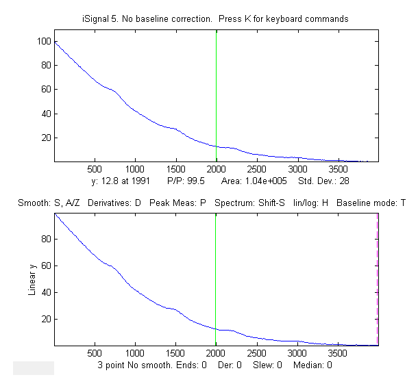
displayed in the upper graph window. The label under the top graph
window shows the value of the signal (y) at the green cursor, the
peak-to-peak (min and max) signal range, the area under the signal,
and the standard deviation within the selected range (the dotted
cursors). Pressing the Q
key prints out a table of the signal information in the command
window.
Signal is measured by placing the green
center cursor on top of the peak
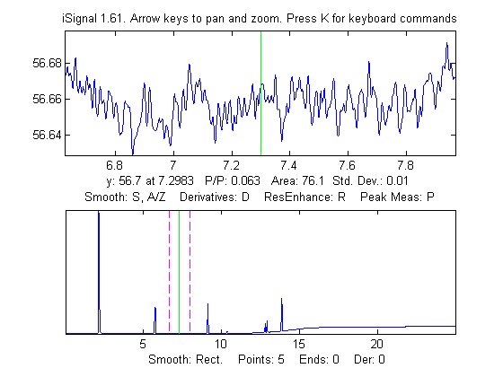
Noise is the standard deviation measured
on a flat portion of the baseline
Signal-to-noise ratio (SNR) measurement of a signal with very high
SNR. Left: The peak height of the largest signal peak is
measured by placing the green center cursor on the largest peak;
peak-to-peak signal=66,000. Right: The noise is measured on a flat
portion of the baseline: standard deviation of noise=0.01,
therefore the SNR=66,000/.01 = 6,600,000
If the optional output arguments maxy, miny, area,
stdev are specified, isignal returns the maximum value
of y, the minimum value of y, the total area under the curve,
and the standard deviation of y, in the selected range displayed
in the upper panel.
Frequency
Spectrum mode
The Frequency Spectrum mode,
toggled on and off by the Shift-S
key, computes the Fourier
frequency spectrum of the segment of the signal displayed in
the upper window and displays it in the lower window (temporarily
replacing the full-signal display). Use the pan and zoom keys to
adjust the region of the signal to be viewed. Press Shift-A to cycle through four
plot modes (linear, semilog X, semilog Y, or log-log) and press Shift-X to toggle between a frequency on the x axis
and time on the
x-axis. All signal processing functions remain active in
the frequency spectrum mode (smooth, derivative, etc) so
you can observe the effect of these functions on the frequency
spectrum of the signal, as in the animated figure on the right.
Press Shift-T to transfer the frequency spectrum to the
signal in the upper panel, so you can pan and zoom and do other
processing and measurements on the frequency spectrum. Press Shift-S again to return to the
normal mode. Spectrum mode is a visible mode, indicated by
the label at the top of the figure. To start off in the
spectrum mode, set the 13th input argument, SpectrumMode, to 1. To save the spectrum as
a new variable, call isignal with the output arguments [pY,Spectrum]:
>> x=0:.1:60; y=sin(x)+sin(10.*x); >>
[pY,Spectrum]=isignal([x;y],30,30,4,3,1,0,0,1,0,0,0,1); >> plot(Spectrum(:,1),Spectrum(:,2)) or
plotit(Spectrum) or isignal(Spectrum);
or ipf(Spectrum); or ipeak(Spectrum);
or whatever.
Shift-Z toggles on and off peak detection and labeling on the
frequency/time spectrum; peaks are labeled with their frequencies.
You can adjust the peak detection parameters in lines 2192-2195 in
version 5; see http://terpconnect.umd.edu/~toh/spectrum/PeakFindingandMeasurement.htm.
The Shift-W command displays the 3D waterfall
spectrum, by dividing up the signal into segments and
computing the power spectrum of each segment. This is
mostly a novelty, but it may be useful for signals whose
frequency spectrum varies over the duration of the signal. You are
asked to choose the number of segments into which to divide the
signal (that is, the number of spectra) and the type of 3D display
(mesh, contour, surface, etc).
Background subtraction
There are two ways to subtract the background from the signal:
automatic and manual. To select an automatic baseline correction
mode, press the T key
repeatedly; it cycles thorough four modes: No baseline
correction, linear baseline subtraction, quadratic baseline
subtraction, flat baseline correction, then back to no
baseline correction. When baseline mode is linear,
a straight-line baseline connecting the two ends of the signal
segment in the upper panel will be automatically
subtracted. When baseline mode is quadratic, a
parabolic baseline connecting the two ends of the signal segment in
the upper panel will be automatically subtracted. The baseline is
calculated by computing a linear (or quadratic) least-squares fit to
the signal in the first 1/10th of the points and the
last 1/10th of the points. Try to adjust the pan and zoom
to include some of the baseline at the beginning and end of the
segment in the upper window, allowing the automatic baseline
subtract gets a good reading of the baseline. The flat baseline
mode is used only for peak fitting. The
calculation of the signal amplitude, peak-to-peak signal, and peak
area are all recalculated based on the baseline-subtracted
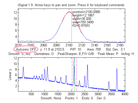
signal in the upper window. If you are measuring peaks superimposed
on a background, the use of the autozero mode will have a big effect
on the measured peak height, width, and area, but very little
effect on the peak x-axis position, as demonstrated by these two
figures.
In addition to the four autozero baseline subtraction modes for peak
measurement, a manually estimated piecewise linear baseline
can be subtractedfrom the entire signal in one operation. The Backspace key starts background
correction operation. In the command window, type in the number
of background points to click and press the Enter key. The cursor changes to
crosshairs; click along the presumed background in the figure
window, starting to the left of the x axis and placing the last
click to the right of the x axis. When the last point is clicked,
the linearly interpolated baseline between those points is
subtracted from the signal. To restore the original background (i.e.
to start over), press the '\'
key (just below the backspace key).
Peak and valley
measurement
The P key toggles off and
on the "peak parabola" mode, which attempts to measure the one peak
(or valley) that is centered in the upper window under the green
cursor by superimposing a least-squares
best-fit parabola, in red, on the center portion of the signal
displayed in the upper window. (Zoom in so that the red overlays
just the top of the peak or the bottom of the valley as closely as
possible). The peak position, height, and width are measured by
least-squares curve fitting of a Gaussian to the central peak over
the segment that is colored red in the upper panel. (Change the pan
and zoom to modify that region; the readings will change as the
segment measured is changed). The "RSquared" value is the
coefficient of determination; the closer to 1.000 the better. The
peak parameters will most accurate if the peaks are Gaussian. Other
peak shapes, or very noisy peaks of any shape, will give only
approximate results. However, the position and height, and area
values are pretty good for any peak shape as long as the "RSquared"
value is at least 0.99. The "SNR" is the signal-to-noise-ratio
of the peak under the green cursor; it's the ratio of the peak
height to the standard deviation of the residuals between the data
and the best-fit line in red. Example shown in the figure on the
right. If the peaks are superimposed on a non-zero background,
subtract the background before measuring peaks, either by using the
autozero mode (T key) or the
multi-point background subtraction (backspace key). Press the R key to print out the peak
parameters in the command window.
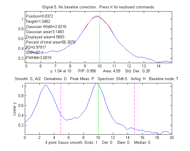
Peak width is actually measured two ways: the
"Gaussian Width" is the width measured by Gaussian curve fitting
(over the region colored in red in the upper panel) and is strictly
accurate only for Gaussian peaks. Version 5.8 (shown below
on the left) adds direct measurement of
the full width at half maximum ('FWHM') of the central
peak in the upper panel (the peak marked by the green
vertical line); this works for peaks of any shape, but it is
computed only for the central peak and only if the half-maximum
points fall within the zoom region displayed in the upper panel
(otherwise it will return NaN). It will not be highly accurate for
very noisy peaks. The Gaussian width will be more accurate for noisy
or sparsely sampled peaks, but only if the peaks are at least
approximately Gaussian. In the example on the right, the peaks are
Lorentzian, with a true with of 3.0, plus added noise. In this case
the measured FWHM (3.002) is more accurate that the Gaussian width
(2.82), especially if a little smoothing is used to reduce the
noise.
Peak
area is also measured two ways: the "Gaussian area"
and the "Total area". The "Gaussian area" is the area under
the Gaussian that is best fit to the center portion of the
signal displayed in the upper window, marked in red. The
"Total area" is the area by the trapezoidal method over the entire
selected segment displayed in the upper window. (The percent of
total area is also calculated). If the portion of the signal
displayed in the upper window is a pure Gaussian with no noise and a
zero baseline, then the two measures should agree almost exactly.
If the peak is not Gaussian in shape, then the total area is
likely to be more accurate, as long as the peak is well separated
from other peaks. If the peaks are overlapped, but have a known
shape, then peak fitting (Shift-F) will give more accurate
peak areas. In the example above on the right, the Lorentzian
peak at x=10 has a true area of 4.488, so in this case the total
area (4.59) is more accurate than the Gaussian area (3.14), but it
is too high because of overlap with the peak at x=3. Curve fitting
both Lorentzians peaks together would yield the most accurate areas.
If the signal is panned slightly left and right, using the left and
right cursor keys or the "[" and "]" keys, the peak parameters
displayed will change slightly due to the noise in the data - the
more noise, the greater the change, as in the example on the left.
If the peak is asymmetrical, as in this example, the peak widths
displayed on one side will be greater that the other side.
In version 5.9 there is an automatic peak finder that is based on
the autopeaks.m
function (activated by the J key); it asks for the peak
density (roughly the number of peaks that fit into the signal
record), then detects, measures, and displays the peak position,
height, and area of all the peaks it detects in the processed signal
currently displayed in the lower panel, plots and number the peaks
as shown on the right and also plots
each peak separately in Figure(2) with peak, tangent, and
valley points marked. (The peak density number controls the peaks
sensitivity - larger numbers cause the routine to detect larger
numbers of narrower peaks, and smaller numbers ignore the fine
structure and looks for broader peaks). It also prints out the peak
detection parameters that it calculates for use by any of the findpeaks... functions.
To return to the usual iSignal display, press any cursor arrow key.
(Shift-J does the same thing for the segment displayed in the
upper window).
Peak
fitting (NEW PROCEDURE in version 5 and later) iSignal has an iterative
curve fitting method performed by peakfit.m. This is the most
accurate method for the measurements of the areas of highly
overlapped peaks. First, center the signal you wish to fit using the
pan and zoom keys (cursor arrow keys), select the baseline mode by
pressing the 'T' key to cycle through the 4
modes. Press the Shift-F
key, then type the desired peak shape by number from the menu
displayed in the Command window (shown below), enter the number of
peaks, enter the number of repeat trial fits (usually 1-10), and
finally click the mouse pointer on the top graph where you think
the peaks might be. A graph of the fit is displayed in Figure
window 2 and a table of results is printed out in the command
window. Version 5 of iSignal can fit many different combinations of
peak shapes and constraints:
Gaussians: y=exp(-((x-pos)./(0.6005615.*width)) .^2) Gaussians with independent positions and
widths.....................1 (default) Exponentially-broadened Gaussian (equal time
constants).............5 Exponentially-broadened equal-width
Gaussian........................8 Fixed-width exponentially-broadened
Gaussian.......................36 Exponentially-broadened Gaussian (independent time
constants)......31 Gaussians with the same
widths......................................6 Gaussians with preset fixed
widths.................................11 Fixed-position
Gaussians...........................................16 Asymmetrical Gaussians with unequal half-widths on
both sides......14 Lorentzians:
y=ones(size(x))./(1+((x-pos)./(0.5.*width)).^2) Lorentzians with independent positions and
widths...................2 Exponentially-broadened
Lorentzian.................................18 Equal-width
Lorentzians.............................................7 Fixed-width
Lorentzian.............................................12 Fixed-position
Lorentzian..........................................17 Gaussian/Lorentzian blend (equal
blends).............................13 Fixed-width Gaussian/Lorentzian
blend..............................35 Gaussian/Lorentzian blend with independent
blends).................33 Voigt profile with equal
alphas).....................................20 Fixed-width Voigt profile with equal
alphas........................34 Voigt profile with independent
alphas..............................30 Logistic: n=exp(-((x-pos)/(.477.*wid)).^2);
y=(2.*n)./(1+n)...........3 Pearson:
y=ones(size(x))./(1+((x-pos)./((0.5.^(2/m)).*wid)).^2).^m....4 Fixed-width
Pearson................................................37 Pearson with independent shape factors,
m..........................32 Breit-Wigner-Fano....................................................15 Exponential pulse:
y=(x-tau2)./tau1.*exp(1-(x-tau2)./tau1)............9 Alpha function:
y=(x-spoint)./pos.*exp(1-(x-spoint)./pos);...........19 Up Sigmoid (logistic function):
y=.5+.5*erf((x-tau1)/sqrt(2*tau2))...10 Down Sigmoid
y=.5-.5*erf((x-tau1)/sqrt(2*tau2))......................23 Triangular...........................................................21
Note: if you have a peak that is an exponentially-broadened Gaussian
or Lorentzian, you can measure both the "after-broadening" height,
position, and width using the P key function, and the
"before-broadening" height, position, and approximate width by
fitting the peak to an exponentially-broadened Gaussian or
Lorentzian model (shapes 5, 8,36, 31, or 18) using the Shift-F
key function. The peak areas will be the same; broadening does not
effect the total peak area.
Polynomial fitting. Shift-o fits a simple polynomial (linear, quadratic, cubic,
etc) to the upper panel segment and displays the coefficients (in
descending powers) and the correlation coefficient R2
Saving the results
To save the processed signal to the disc as an x,y matrix in mat
format, press the 'o' key, then type in the desired file name into
the "File name" field, then press Enter or click Save.
To load into the workspace, type "load" followed by the file name
you typed. The processed signal will be saved in a matrix called
"Output"; to plot the processed data, type
"plot(Output(:,1),Output(:,2))". Other keystroke
controls
The Shift-G key toggles on and off a temporary grid on the
upper and lower panel plots. The L
key toggles off and on the Overlay mode, which shows the original
signal as a dotted line overlaid on the current processed signal,
for the purposes of comparison. Shift-B opens Figure window
2 and plots the original signal in the upper panel and the processed
signal in the lower panel (graphic).
The Tab key restores the
original signal and cursor settings. The ";" key sets the selected region to zero (to
eliminate artifacts and spikes). The "-" (minus sign) key is used to
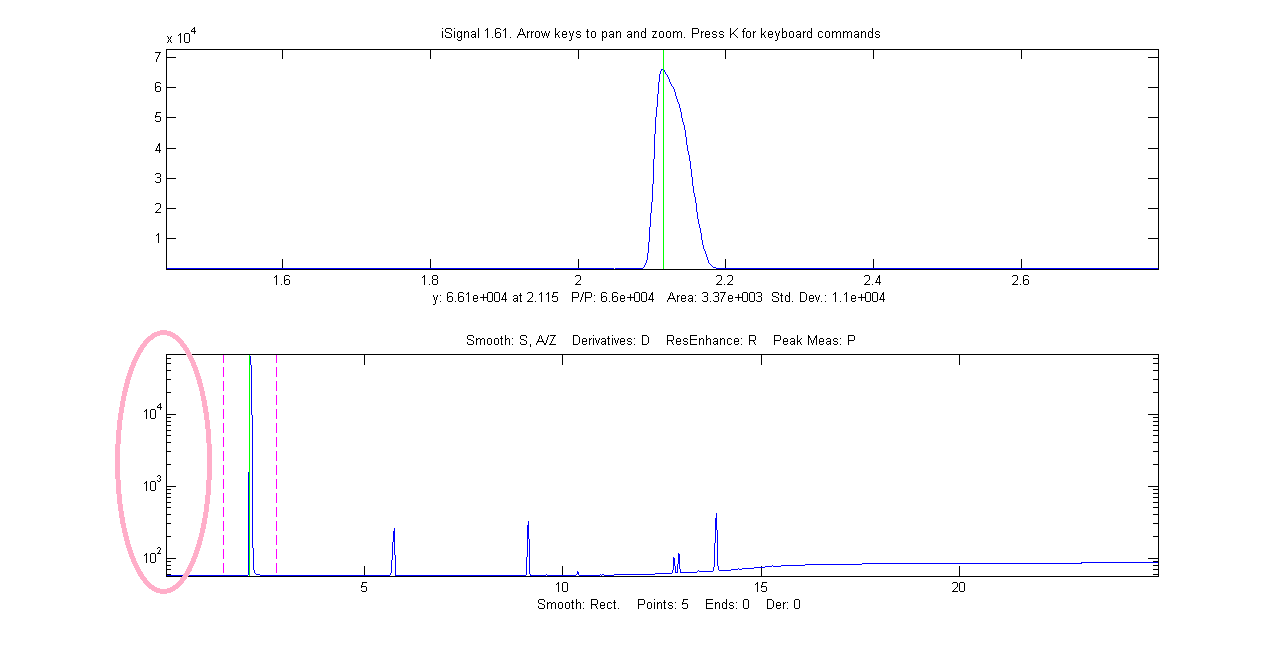
negate the signal (flip + for -). Press H to toggle display of semilog y
plot in the lower window, which is useful for signals with very wide
dynamic range, as in the example in the figures below (zero and
negative points are ignored in the log plot). Press '+' key to take the
absolute value of the entire signal (and follow this by a smooth to create an amplitude modulation
"detector"). In version 5.7, Shift-L replaces the signal
with the processed version of itself, for the purpose of applying
more passes of different widths of smoothing or higher orders of
differentiation. In version 5.95, the ^ (Shift-6) raises the
signal to the specified power. To reverse this, simply raise to the
reciprocal power. See Power
transform method of peak sharpening.
Linear y-axis mode
Log y mode (H key)
The C key condenses the
signal by the specified factor n, replacing each group of n points
with their average (n must be an integer, such as 2,3, 4, etc). The I key replaces the signal with a
linearly interpolated version containing m data
points. This can be used either to increase or decrease the x-axis
interval of the signal or to convert unevenly spaced values to
evenly spaced values. After pressing C or I, you
must type in the value of n or m respectively.
You can press Shift-C, then click on the graph to print out
the x,y coordinates of that point. This works on both the
upper and lower panels, and on the frequency spectrum as well. Playing data as audio.
Press Spacebar or Shift-P to play the segment of
the signal displayed in the upper window as audio through the
computer's sound output. Press Shift-R to set the sampling
rate - the larger the number the shorter and higher-pitched will be
the sound. The default rate is 44000Hz. Sounds or music files in WAV
format can be loaded into Matlab using the built-in "wavread"
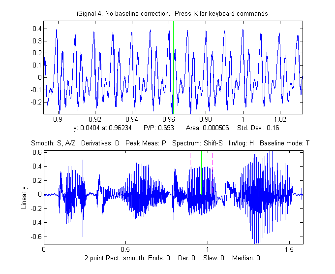
function. The example on the right shows a 1.5825 sec duration audio
recording of the phrase "Testing, one, two, three" recorded at 44000
Hz, saved in WAV format (link),
loaded into iSignal and zoomed in on the "oo" sound in the word
"two". Press Spacebar to play the selected sound; press Shift-S
to display the frequency spectrum
of the selected region, and press Shift-Z to label the peaks
in the frequency spectrum with their frequencies (graphic).
Press Shift-R and type 44000 to set the sampling rate. This
recorded sound example allows you to experiment with the effect of
smoothing, differentiation, and interpolation on the sound of
recorded speech. Interestingly, different degrees of smoothing and
differentiation will change the timbre of the
voice but has little effect on the intelligibility. This is
because the sequence of frequency components in the signal is not
shifted in pitch or in time but merely changed in amplitude by
smoothing and differentiation. Even computing the absolute value
(+ key), which effectively doubles the fundamental frequency, does
not make the sound unintelligible.
Shift-Ctrl-F transfers the current signal to
Interactive Peak Fitter (ipf.m) and Shift-Ctrl-P
transfers the current signal to Interactive Peak Detector
(iPeak.m), if those functions are installed in your Matlab path.
Press K to see all the
keyboard commands.
EXAMPLE 1:
Single input argument; data in a two columns of a matrix [x;y] or in
a single y vector
>> isignal(y);
>> isignal([x;y]);
EXAMPLE 2: Two input
arguments. Data in separate x and y vectors.
>> isignal(x,y);
EXAMPLE 3: Three or four
input arguments. The last two arguments specify the initial values of pan (xcenter) and
zoom (xrange) in the last two input arguments. Using data in the ZIP
file:
>> load data.mat
>> isignal(DataMatrix,180,40); or
>> isignal(x,y,180,40);
EXAMPLE 4: As above, but
additionally specifies initial values of SmoothMode, SmoothWidth,
ends, and DerivativeMode in the last four input arguments.
>> isignal(DataMatrix,180,40,2,9,0,1); EXAMPLE 5: As above, but
additionally specifies initial values of the peak sharpening
parameters Sharpen, Sharp1, and Sharp2 in the last three input
arguments. Press the E
key to toggle sharpening on and off for comparison.
>>
isignal(DataMatrix,180,40,4,19,0,0,1,51,6000);
EXAMPLE 6:
Using the built-in "humps" function: >>
x=[0:.005:2];y=humps(x);Data=[x;y];
4th derivative of the peak at x=0.9: >>
isignal(Data,0.9,0.5,1,3,1,4); (shown on the right ==>)
Peak sharpening applied to the peak at x=0.3: >>
isignal(Data,0.3,0.5,1,3,1,0,1,220,5400);
(Press 'E' key to toggle sharpening ON/OFF to compare)
EXAMPLE 7: Measurement of
peak area. This example generates four Gaussian peaks, all
with the exact same peak height (1.00) and area (1.77). The first
peak (at x=4) is isolated, the second peak (x=9) is slightly
overlapped with the third one, and the last two peaks (at x= 13 and
15) are strongly overlapped. To measure the area under a peak
using the perpendicular drop method, position the dotted red marker
lines at the minimum between the overlapped peaks.
Greater accuracy in peak area
measurement using iSignal can be obtained by using the peak sharpening function to
reduce the overlap between the peaks. This reduces the peak
widths, increases the peak heights, but has no effect on the
peak areas.
EXAMPLE 8: Single peak with random spikes (shown in the figure on the right).
Compare smoothing vs spike filter (M key) and slew rate
limit (~ key) to remove spikes.
x=-5:.01:5;
y=exp(-(x).^2);
for n=1:1000,
 if randn()>2,y(n)=rand()+y(n),
 end,
end;
isignal(x,y);
EXAMPLE 9:Weak peaks on a strong baseline.
The demo script isignaldemo2
(shown on the left) creates a test signal containing four
peaks with heights 4, 3, 2, 1, with equal widths,
superimposed on a very strong curved baseline, plus added
random white noise. The objective is to extract a measure
that is proportional to the peak height but independent of
the baseline strength. Suggested approaches: (a) Use
automatic or manual baseline subtraction to remove the
baseline, measure peaks with the P-P measure in the upper
panel; or (b) use differentiation (with smoothing) to
suppress the baseline; or (c) use curve fitting (Shift-F),
with baseline correction (T), to measure peak height.
After running the script, you can press Enter to
have the script perform an automatic 3rd derivative
calibration, performed by lines 56 to 74. As indicated in
the script, you can change several of the constants; search
for the word "change". (To use the derivative method, the width
of the peaks must all be equal and stable, but the peak
positions may vary within limits, set by the Xrange
for each peak in lines 61-67). You must have isignal.m and
plotit.m installed.
EXAMPLE 10:
Direct entry into frequency spectrum mode, plotting returned
frequency spectrum.
>> x=0:.1:60; y=sin(x)+sin(10.*x); >>
[pY,SpectrumOut]=isignal([x;y],30,30,4,3,1,0,0,1,0,0,0,1); >> plot(SpectrumOut)
EXAMPLE 11:
The demo script demoisignal.m
is a self-running demo that requires iSignal 4.2 or later
and the latest version of plotit.m
to be installed.
EXAMPLE
12: Here's a simple example of a
very noisy signal with lots of high-frequency
(blue) noise obscuring a perfectly good peak in
the center at x=150, height=1e-4; SNR=90.
First, download
NoisySignal
into
the Matlab path, then execute these statements:
Use the A and Z keys to increase and decrease the
smooth width, and the S key to cycle through the available
smooth type. Hint: use the Gaussian smooth and keep increasing the
smooth width.
Zoom in on the peak in the center, press P to enter the peak
mode, and it will display the characteristics of the peak in
the upper left.
KEYBOARD CONTROLS (Version
8): Pan left and
right..........Coarse pan: <
and >
Fine
pan: left and right cursor arrows
Nudge:
[ and ]
Zoom in and out.............Coarse zoom: / and "
Fine
zoom: up and down cursor arrows
Resets pan and zoom.........ESC
Select entire signal........Ctrl-A Display Grid (on/off).......Shift-G
Temporarily displays grid on
the plots Adjust smooth width.........A,Z (A=>more, Z=>less)
Set smooth width vector.....Shift-Q for
segmented smooth Adjust
smooth type..........S
(cycles through None, Rectangular, Triangle, Gaussian,and Savitzky-Golay)
Toggle smooth ends..........X (0=ends zeroed 1=ends smoothed (slower)
Symmetrize
mode
Shift-Y toggles off and on
Adjust SymFactor............1,2:
decrease,increase by 10% Shift-1,Shift-2: decrease,increase by 1%
ConV/deconVolution mode.....Shift-V presents
conv/deconv menu
Adjust width................3,4:
decrease,increase by 10% Shift-3,Shift-4: decrease,increase by 1%
Adjust derivative order.....D/Shift-D Increase/Decrease
derivative
order
Toggle peak sharpening......E (0=OFF 1=ON)
Sharpening for Gaussian.....Y Set sharpen settings for Gaussian
Sharpening for Lorentzian...U Set sharpen settings for Lorentzian
Adjust sharp1...............F,V
F=>sharper, V=>less sharpening
Adjust sharp2 ............G,B G=>sharper, B=>less sharpening
Slew rate limit (0=OFF).....~ Largest allowed y change between points
Spike filter width (0=OFF)..Mmedian
filter eliminates sharp spikes
Toggle peak parabola........P fits parabola to center, labels vertex
Fits peak in upper window...Shift-F (Asks for shape, number of peaks,
Number of trials, etc)
Fit polynomial..............Shift-o Fits
polynomial to data in
upper panel
Find peaks in lower panel...J (Asks for Peak
Density)
Find peaks in upper panel...Shift-J (Asks for
Peak Density)
Spectrum mode on/off........Shift-S (Shift-A
and Shift-X to change
axes)
Peak labels on spectrum.....Shift-Z in
spectrum mode
Display Waterfall spectrum..Shift-W
Allows choice of mesh, surf,
contour, or pcolor
Transfer power spectrum.....Shift-T
Replaces signal with power
spectrum
Click graph to print x,y....Shift-C
Click graph to print coordinates
Lock in current processing..Shift-L
Replace signal with processed
version
Power transform method......^ (Shift-6) Raises
the signal to the specified power. Print peak report...........R prints position,
height, width, area
Toggle overlay mode.........L Overlays original signal as dotted line
Display current signals.....Shift-B
Original (top) vs Processed
(bottom)
Toggle log y mode...........H semilog plot in lower window
Cycle baseline mode.........T none,
linear, quadratic, or flat
baseline
mode
Restores original signal....Tab key resets to original signal
and modes
Baseline subtraction........Backspace, then click baseline at
multiple points
Restore background..........\ to cancel previous background
subtraction
Invert signal...............- Invert (negate) the signal (flip + / -)
Remove offset...............0 (zero) set minimum signal to zero
Sets region to zero.........; sets selected region to zero.
Absolute value..............+ Computes absolute
value of entire
signal
Condense signal.............C Condense oversampled signal by
factor N
Interpolate signal..........i Interpolate (re-sample) to N points
Print keyboard commands.....K prints this list
Print signal report.........Q prints signal info and current
settings
Print isignal arguments.....W prints isignal (current arguments)
Save output to disk.........O as .mat file with processed signal
matrix and (in spectrum mode) the
frequency spectrum.
Play signal as sound........Spacebar or
Shift-P Play upper panel segment through computer sound system
Set sound sample rate.......Shift-R for the
Shift-P command.
Switch to ipf.m.............Shift-Ctrl-FTransfer current signal
to
Interactive Peak Fitter Switch to
iPeak.............Shift-Ctrl-PTransfer current signal
to
Interactive Peak Detector
ProcessSignal, a Matlab/Octave
command-line function that performs smoothing and
differentiation on the time-series data set x,y (column or row
vectors). Type "help ProcessSignal". Returns the processed
signal as a vector that has the same shape as x, regardless of
the shape of y. The syntax is
Processed=ProcessSignal(x, y, DerivativeMode, w, type, ends,
Sharpen, factor1, factor2, SlewRate, MedianWidth)
December, 2021. This page is part of "A
Pragmatic Introduction to Signal Processing", created
and maintained by Prof.
Tom O'Haver , Department of Chemistry and Biochemistry, The
University of Maryland at College Park. Comments, suggestions and
questions should be directed to Prof. O'Haver at toh@umd.edu.
 ing
the entire signal, and the upper half showing a selected portion
controlled by the pan and zoom keys (the four cursor arrow keys),
with the initial pan and zoom settings optionally controlled by
input arguments 'xcenter'
and 'xrange', respectively.
Other keystrokes allow you to control the smooth type, width, and
ends treatment, the derivative order (0th through 5th),
and peak sharpening. (The initial values of all these parameters can
be passed to the function via the optional input arguments SmoothMode, SmoothWidth, ends, DerivativeMode, Sharpen,
Sharp1, Sharp2, SlewRate, and MedianWidth.
See the examples below). Press K
to see all the keyboard commands. Note:
Make sure you don't click on the "Show Plot Tools" button in
the toolbar above the figure; that will
disable normal program functioning. If you do; close the
Figure window and start again.
ing
the entire signal, and the upper half showing a selected portion
controlled by the pan and zoom keys (the four cursor arrow keys),
with the initial pan and zoom settings optionally controlled by
input arguments 'xcenter'
and 'xrange', respectively.
Other keystrokes allow you to control the smooth type, width, and
ends treatment, the derivative order (0th through 5th),
and peak sharpening. (The initial values of all these parameters can
be passed to the function via the optional input arguments SmoothMode, SmoothWidth, ends, DerivativeMode, Sharpen,
Sharp1, Sharp2, SlewRate, and MedianWidth.
See the examples below). Press K
to see all the keyboard commands. Note:
Make sure you don't click on the "Show Plot Tools" button in
the toolbar above the figure; that will
disable normal program functioning. If you do; close the
Figure window and start again. vector in
two ways: at the prompt you can (a) enter the number of
segments (then you'll be prompted to enter the smooth widths in the
first and last segments, and the computer will calculate integer
values of smooth widths that are evenly divided between the
specified first and last values, or (b) type in the smooth width
vector directly including the square brackets, e.g. [1 3 3
9]. In either case, subsequently adjusting the smooth width with the
A and Z keys will vary all the segments by
the same percentage factor. (To return to an ordinary single segment
smooth, enter 1 as the number of segments). Picture on right.
vector in
two ways: at the prompt you can (a) enter the number of
segments (then you'll be prompted to enter the smooth widths in the
first and last segments, and the computer will calculate integer
values of smooth widths that are evenly divided between the
specified first and last values, or (b) type in the smooth width
vector directly including the square brackets, e.g. [1 3 3
9]. In either case, subsequently adjusting the smooth width with the
A and Z keys will vary all the segments by
the same percentage factor. (To return to an ordinary single segment
smooth, enter 1 as the number of segments). Picture on right.

 ne setting will not
be optimum for all the peaks). You can fine-tune the sharpening
with the F/V and G/B keys and the smoothing
with the A/Z keys.
ne setting will not
be optimum for all the peaks). You can fine-tune the sharpening
with the F/V and G/B keys and the smoothing
with the A/Z keys.  ignal has
peaks that are exponentially broadened, you can remove that
broadening, and increase the symmetry of the peaks, by the weighted
first-derivative addition technique. Press Shift-Y and
enter an estimated weighting factor (e.g., start with the width of
the peak), then press the "1" and "2" keys to change
weighting factor by 10% and the "Shift-1" and "Shift-2"
keys to change by 1%. Increase the factor until the baseline after
the peak goes negative, then increase it slightly so that it is as
low as possible but not negative. Adjust the smoothing to
control the noise (the Savitsky-Golay smooth is ideal here). The
result is narrower, taller peaks, but with the peak areas. It has
the same effect as deconvoluting the exponential function from the
broadened signal, but it is faster and simpler. It the peaks tail to
the left rather than the right, use a negative weighting
factor. To cancel the effect, press Shift-Y
and set the time constant to zero. Run the script iSignalSymmTest.m for a example
signal with two overlapping exponentially broadened Gaussians. The
graphic on the left shows a real-data example, after which the L
key was pressed to overlay and compare the de-tailed peaks (in
blue) with the original signal (in cyan). If desired, and if the
signal-to-noise ratio is not too poor, the de-tailed peaks can be
further sharpened using the even-derivative technique (E key,
previous section).
ignal has
peaks that are exponentially broadened, you can remove that
broadening, and increase the symmetry of the peaks, by the weighted
first-derivative addition technique. Press Shift-Y and
enter an estimated weighting factor (e.g., start with the width of
the peak), then press the "1" and "2" keys to change
weighting factor by 10% and the "Shift-1" and "Shift-2"
keys to change by 1%. Increase the factor until the baseline after
the peak goes negative, then increase it slightly so that it is as
low as possible but not negative. Adjust the smoothing to
control the noise (the Savitsky-Golay smooth is ideal here). The
result is narrower, taller peaks, but with the peak areas. It has
the same effect as deconvoluting the exponential function from the
broadened signal, but it is faster and simpler. It the peaks tail to
the left rather than the right, use a negative weighting
factor. To cancel the effect, press Shift-Y
and set the time constant to zero. Run the script iSignalSymmTest.m for a example
signal with two overlapping exponentially broadened Gaussians. The
graphic on the left shows a real-data example, after which the L
key was pressed to overlay and compare the de-tailed peaks (in
blue) with the original signal (in cyan). If desired, and if the
signal-to-noise ratio is not too poor, the de-tailed peaks can be
further sharpened using the even-derivative technique (E key,
previous section). from a group of
three overlapping Lorentzians in a effort to narrow the peaks. The
screen shows the signal zoomed to the middle peak (top panel). The
entire signal is shown in the bottom panel. The animation shows
what happens when you increase the width of the deconvolution
Lorentzian ("Vwidth", displayed at the bottom of the lower panel)
from 0.16 to 2.5 and then back drown to around 2. (I do that with
the 3 and 4 keys). Watch the close-up of the center peak in the
upper panel, which also measures the peak position, height, with
and area continuously. The height goes up and the width goes down.
How far can you go with this? In many experimental domains,
the signal is expected to be positive, except for
instances where random noise on the baseline may make the signal
occasionally slightly negative. If you increase the deconvolution
width too far, the peaks will develop negative dips on their sides
and will become excessively noisy. That sets an upper limit to the
deconvolution with that can be employed, but that has to be
determined experimentally on a case-by-case basis, guided by the
needs of the experimenter. For a real-data example, see Deconvolution.html#Data658.
Note: in cases where the peak widths within a group of peaks are
substantially different, you can use segmented deconvolution.
from a group of
three overlapping Lorentzians in a effort to narrow the peaks. The
screen shows the signal zoomed to the middle peak (top panel). The
entire signal is shown in the bottom panel. The animation shows
what happens when you increase the width of the deconvolution
Lorentzian ("Vwidth", displayed at the bottom of the lower panel)
from 0.16 to 2.5 and then back drown to around 2. (I do that with
the 3 and 4 keys). Watch the close-up of the center peak in the
upper panel, which also measures the peak position, height, with
and area continuously. The height goes up and the width goes down.
How far can you go with this? In many experimental domains,
the signal is expected to be positive, except for
instances where random noise on the baseline may make the signal
occasionally slightly negative. If you increase the deconvolution
width too far, the peaks will develop negative dips on their sides
and will become excessively noisy. That sets an upper limit to the
deconvolution with that can be employed, but that has to be
determined experimentally on a case-by-case basis, guided by the
needs of the experimenter. For a real-data example, see Deconvolution.html#Data658.
Note: in cases where the peak widths within a group of peaks are
substantially different, you can use segmented deconvolution.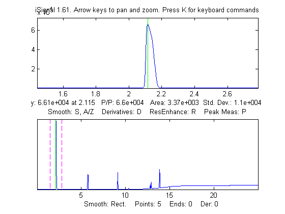

 Peak
area is also measured two ways: the "Gaussian area"
and the "Total area". The "Gaussian area" is the area under
the Gaussian that is best fit to the center portion of the
signal displayed in the upper window, marked in red. The
"Total area" is the area by the trapezoidal method over the entire
selected segment displayed in the upper window. (The percent of
total area is also calculated). If the portion of the signal
displayed in the upper window is a pure Gaussian with no noise and a
zero baseline, then the two measures should agree almost exactly.
If the peak is not Gaussian in shape, then the total area is
likely to be more accurate, as long as the peak is well separated
from other peaks. If the peaks are overlapped, but have a known
shape, then peak fitting (Shift-F) will give more accurate
peak areas. In the example above on the right, the Lorentzian
peak at x=10 has a true area of 4.488, so in this case the total
area (4.59) is more accurate than the Gaussian area (3.14), but it
is too high because of overlap with the peak at x=3. Curve fitting
both Lorentzians peaks together would yield the most accurate areas.
If the signal is panned slightly left and right, using the left and
right cursor keys or the "[" and "]" keys, the peak parameters
displayed will change slightly due to the noise in the data - the
more noise, the greater the change, as in the example on the left.
If the peak is asymmetrical, as in this example, the peak widths
displayed on one side will be greater that the other side.
Peak
area is also measured two ways: the "Gaussian area"
and the "Total area". The "Gaussian area" is the area under
the Gaussian that is best fit to the center portion of the
signal displayed in the upper window, marked in red. The
"Total area" is the area by the trapezoidal method over the entire
selected segment displayed in the upper window. (The percent of
total area is also calculated). If the portion of the signal
displayed in the upper window is a pure Gaussian with no noise and a
zero baseline, then the two measures should agree almost exactly.
If the peak is not Gaussian in shape, then the total area is
likely to be more accurate, as long as the peak is well separated
from other peaks. If the peaks are overlapped, but have a known
shape, then peak fitting (Shift-F) will give more accurate
peak areas. In the example above on the right, the Lorentzian
peak at x=10 has a true area of 4.488, so in this case the total
area (4.59) is more accurate than the Gaussian area (3.14), but it
is too high because of overlap with the peak at x=3. Curve fitting
both Lorentzians peaks together would yield the most accurate areas.
If the signal is panned slightly left and right, using the left and
right cursor keys or the "[" and "]" keys, the peak parameters
displayed will change slightly due to the noise in the data - the
more noise, the greater the change, as in the example on the left.
If the peak is asymmetrical, as in this example, the peak widths
displayed on one side will be greater that the other side.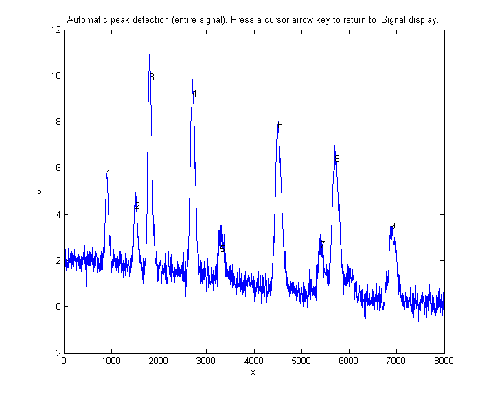 based on
the autopeaks.m
function (activated by the J key); it asks for the peak
density (roughly the number of peaks that fit into the signal
record), then detects, measures, and displays the peak position,
height, and area of all the peaks it detects in the processed signal
currently displayed in the lower panel, plots and number the peaks
as shown on the right and also plots
each peak separately in Figure(2) with peak, tangent, and
valley points marked. (The peak density number controls the peaks
sensitivity - larger numbers cause the routine to detect larger
numbers of narrower peaks, and smaller numbers ignore the fine
structure and looks for broader peaks). It also prints out the peak
detection parameters that it calculates for use by any of the findpeaks... functions.
To return to the usual iSignal display, press any cursor arrow key.
(Shift-J does the same thing for the segment displayed in the
upper window).
based on
the autopeaks.m
function (activated by the J key); it asks for the peak
density (roughly the number of peaks that fit into the signal
record), then detects, measures, and displays the peak position,
height, and area of all the peaks it detects in the processed signal
currently displayed in the lower panel, plots and number the peaks
as shown on the right and also plots
each peak separately in Figure(2) with peak, tangent, and
valley points marked. (The peak density number controls the peaks
sensitivity - larger numbers cause the routine to detect larger
numbers of narrower peaks, and smaller numbers ignore the fine
structure and looks for broader peaks). It also prints out the peak
detection parameters that it calculates for use by any of the findpeaks... functions.
To return to the usual iSignal display, press any cursor arrow key.
(Shift-J does the same thing for the segment displayed in the
upper window).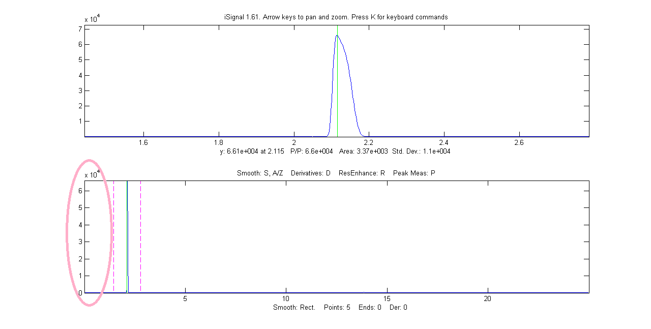
 Playing data as audio.
 of pan (xcenter) and
zoom (xrange) in the last two input arguments. Using data in the ZIP
file:
of pan (xcenter) and
zoom (xrange) in the last two input arguments. Using data in the ZIP
file:  >>
x=[0:.005:2];y=humps(x);Data=[x;y];
>>
x=[0:.005:2];y=humps(x);Data=[x;y];
 EXAMPLE 9:
Weak peaks on a strong baseline.
EXAMPLE 9:
Weak peaks on a strong baseline.

