(1) a command line version (peakfit.m) for Matlab or Octave, Matlab File Exchange "Pick of the Week". The current version number is 9.9, July 2021.The difference between them is that peakfit.m is completely controlled by command-line input arguments and returns its information via command-line output arguments; ipf.m allows interactive control via keypress commands. For automating the fitting of large numbers of signals, peakfit.m is better (see Appendix X for an example); but ipf.m is best for exploring signals to determine the optimum fitting range, peak shapes, number of peaks, baseline correction mode, etc. Otherwise they have similar curve-fitting capabilities. The basic built-in peak shape models available are illustrated in this graphic; custom peak shapes can be added. See Notes and Hints for more information and useful suggestions.
(2) a keypress operated interactive version ipf.m, or its Octave version ipfoctave. The current version number is 13.5.
Peakfit.m is a user-defined command window peak fitting function for Matlab or Octave, usable from a remote terminal. It is written as a self-contained function in a single m-file. (To view of download, click peakfit.m). It takes data in the form of a 2 x n matrix that has the independent variables (X-values) in row 1 and the dependent variables (Y-values) in row 2, or as a single dependent variable vector. The syntax is [FitResults, GOF, baseline, coeff, residuals, xi, yi, BootResults] = peakfit(signal, center, window, NumPeaks, peakshape, extra, NumTrials, start, BaselineMode, fixedparameters, plots, bipolar, minwidth, DELTA, clipheight)). Only the first input argument, the data matrix, is absolutely required; there are default values for all other inputs. All the input and output arguments are explained below.

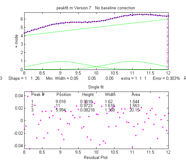
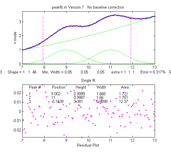
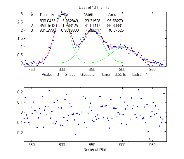
The screen display is shown on the right; the upper panel shows the data as blue dots, the combined model as a red line (ideally overlapping the blue dots), and the model components as green lines. The dotted magenta lines are the first-guess peak positions for the last fit. The lower panel shows the residuals (difference between the data and the model).
You can download a ZIP file
containing peakfit.m, DemoPeakFit.m,
ipf.m, Demoipf.m, some sample data for testing, and
a test script (testpeakfit.m or autotestpeakfit.m) that runs
all the examples sequentially to test for proper operation.
For a discussion of the accuracy and precision of peak
parameter measurement using peakfit.m, click here.
The peakfit.m
functionality can also be accessed by the
keypress-operated interactive functions ipf.m, iPeak.m,
and iSignal.m. all of which contain peakfit.m as a
sub-function.
Latest version 9.9: July 13, 2021, Fixed bug
in Voigt (shapes 20 and 30) and added missing function for
Gompertz, shape 43.
Peakfit.m can be called with several optional additional command line arguments. All input arguments (except the signal itself) can be replaced by zeros to use their default values.
peakfit(signal);
Performs an iterative least-squares fit of a single
unconstrained Gaussian peak to the entire data matrix "signal",
which has x values in row 1 and Y values in row 2 (e.g. [x y]) or
which may be a single signal vector (in which case the data points
are plotted against their index numbers on the x axis).
peakfit(signal,center,window);
Fits a single unconstrained Gaussian peak to a portion of
the matrix "signal". The portion is centered on the x-value
"center" and has width "window" (in x units).
In this and in all following
examples, set "center" and "window" both to 0 to fit the
entire signal.
peakfit(signal,center,window,NumPeaks);
"NumPeaks" = number of peaks in the model (default is 1 if
not specified).
peakfit(signal,center,window,NumPeaks,peakshape);
Number or vector that specifies the peak shape(s) of the
model: 1=unconstrained Gaussian, 2=unconstrained
Lorentzian, 3=logistic distribution, 4=Pearson,
5=exponentially broadened Gaussian; 6=equal-width
Gaussians, 7=equal-width
Lorentzians, 8=exponentially broadened equal-width
Gaussians, 9=exponential pulse, 10= up-sigmoid
(logistic function), 11=fixed-width
Gaussians, 12=fixed-width
Lorentzians, 13=Gaussian/Lorentzian
blend; 14=bifurcated Gaussian, 15=Breit-Wigner-Fano
resonance; 16=Fixed-position
Gaussians; 17=Fixed-position Lorentzians; 18=exponentially
broadened Lorentzian; 19=alpha function; 20=Voigt
profile; 21=triangular; 23=down-sigmoid; 25=lognormal
distribution; 26=linear baseline
(see Example 28); 28=polynomial (extra=polynomial order;
Example 30); 29=articulated linear segmented (see Example
29); 30=independently-variable alpha Voigt ; 31=independently-variable
time constant ExpGaussian; 32=independently-variable
Pearson; 33=independently-variable Gaussian/Lorentzian
blend; 34=fixed-width Voigt; 35=fixed-width
Gaussian/Lorentzian blend; 36=fixed-width
exponentially-broadened Gaussian; 37=fixed-width Pearson;
38= independently-variable time constant ExpLorentzian; 39=
alternative independently-variable time constant ExpGaussian
(see Example 39 below); 40=sine wave; 41=rectangle;
42=flattened Gaussian; 43=Gompertz function (3
parameter logistic: Bo*exp(-exp((Kh*exp(1)/Bo)*(L-t)+1)));
44=1-exp(-k*x); 45: Four-parameter logistic y =
maxy*(1+(miny-1)/(1+(x/ip)^slope)); 46=quadratic baseline
(see Example 38); 47=blackbody emission; 48=equal-width
exponential pulse; 49=Pearson IV (4 varibles); 50=multilinear
regression (known peak positions and widths).
The function ShapeDemo demonstrates most of the basic peak shapes graphically, showing the variable-shape peaks as multiple lines.
Note 1: "unconstrained"
simply means that the position, height, and width of each
peak in
the model can vary independently of the other peaks, as
opposed to the equal-width, fixed-width, or fixed position
variants. Shapes 4, 5, 13, 14, 15, 18, 20, and 34-37 are
are constrained to the same shape constant; shapes
30-33
are completely unconstrained in position, width and
shape; their shape variables are determined by
iteration.
Note 2: The
value of the shape constant "extra" defaults to 1 if not specified
in input arguments.
Note 3: The peakshape argument can be a vector of
different shapes for each peak, e.g. [1 2 1] for three peaks
in a Gaussian, Lorentzian, Gaussian sequence. (The next input
argument, 'extra', must be a vector of the same length as
'peakshape'. See Examples 24, 25, 28 and
38, below.
peakfit(signal,center,window,NumPeaks,peakshape,extra)
Specifies the value of 'extra', used in the Pearson,
exponentially-broadened Gaussian, Gaussian/Lorentzian
blend, bifurcated Gaussian, and Breit-Wigner-Fano
shapes to fine-tune the peak shape. The value of "extra"
defaults to 1 if not specified in input arguments. In version 5,
'extra' can be a vector of different extra values for each peak).
peakfit(signal,center,window,NumPeaks,peakshape,
extra, NumTrials);
Restarts the fitting process "NumTrials" times with
slightly different start values and selects the best one
(with lowest fitting error). NumTrials can be any positive integer
(default is 1). In may cases, NumTrials=1 will be sufficient, but
if that does not give consistent results, increase NumTrials until
the result are stable.
peakfit(signal,center,window,NumPeaks,peakshape,extra,
NumTrials, start)
Specifies the first guesses vector "firstguess" for the
peak positions and widths, e.g. start=[position1 width1 position2
width2 ...]. Only necessary on difficult cases, especially
when there are a lot of adjustable variables. The start vector can
be the approximate average values based on your experience, or it
can be calculated from a previous simpler fit, as in this example.
If you leave this off, or set start=0, the program will generate
its own start values (which is often good enough).
peakfit(signal,center,window,NumPeaks,peakshape,extra,
NumTrials, start, BaselineMode)
As above, but "BaselineMode" sets the baseline correction mode
in the last argument: BaselineMode=0
(default) does not subtract
baseline from data segment;. BaselineMode=1 interpolates a linear
baseline from the edges of the data segment and subtracts it
from the signal (assumes that the peak
returns to the baseline at the edges of the signal);
BaselineMode=2, like mode 1 except that
it computes a quadratic curved baseline; BaselineMode=3
compensates for a flat baseline without reference to
the signal itself (does not require that the signal return to
the baseline at the edges of the signal, as does modes 1 and 2).
Coefficients of the polynomial baselines are returned in the
third output argument "baseline".
peakfit(signal,0,0,0,0,0,0,0,2)
Use zeros as placeholders to use the default values of
input arguments. In this case, BaselineMode is set to 2, but all
others are the default values.
Example
8. As
above,
returns the vector xi containing 600 interpolated x-values for
the model peaks and the matrix yi containing the y values of
each model peak at each xi. Type plot(xi,yi(1,:)) to plot peak 1 or plot(xi,yi,xi,sum(yi)) to plot all the model
components and the total model (sum of components).
> [FitResults, GOF,
baseline, coeff, residuals,xi,yi]=
peakfit(smatrix,.4,.7,2,1,0,10);
> figure(2):clf;plot(xi,yi,xi,sum(yi))
Example 9. Fitting a single
unconstrained Gaussian on a linear background, using the linear
BaselineMode mode (9th input argument = 1)
>>x=[0:.1:10]';y=10-x+exp(-(x-5).^2);peakfit([x
y],5,8,0,0,0,0,0,1)
Example 10. Fits a group of three peaks near x=2400 in DataMatrix3 with three equal-width exponentially-broadened Gaussians.
>> load DataMatrix3
>>
[FitResults,FitError]= peakfit(DataMatrix3,2400,440,3,8,31,1)
Peak
Position Height
Width Peak area
1
2300.5 0.82546
60.535 53.188
2
2400.4 0.48312
60.535 31.131
3
2500.6 0.84799
60.535 54.635
FitError = 0.19975
Example
11. Example
of an unstable fit to a signal consisting of two unconstrained
Gaussian peaks of equal height (1.0). The peaks are too highly
overlapped for a stable fit, even though the fit error is
small and the residuals are unstructured. Each time you
re-generate this signal, it gives a different fit, with the
peaks heights varying about 15% from signal to signal.
>> x=[0:.1:10]';
y=exp(-(x-5.5).^2) + exp(-(x-4.5).^2) + .01*randn(size(x));
[FitResults,FitError]= peakfit([x y],5,19,2,1)
Peak
Position Height
Width Peak area
1
4.4059 0.80119 1.6347
1.3941
2
5.3931 1.1606
1.7697 2.1864
FitError = 0.598
Much more stable results can be
obtained using the equal-width Gaussian model (peakfit([x y],5,19,2,6)),
but that is justified only if the experiment is
legitimately expected to yield peaks of equal width. See http://terpconnect.umd.edu/~toh/spectrum/CurveFittingC.html#Peak_width_constraints.
Example 12. Baseline correction. Demonstration of the four BaselineMode modes, for a single Gaussian on large baseline, with position=10, height=1, and width=1.66. The BaselineMode mode is specified by the 9th input argument (0,1,2, or 3).
BaselineMode=0 means to ignore the baseline (default mode if not specified). In this case, this leads to large errors.
>> x=8:.05:12;y=1+exp(-(x-10).^2);
>> [FitResults,FitError,baseline]=peakfit([x;y],0,0,1,1,0,1,0,0)
FitResults =
1 10 1.8561 3.612 5.7641
FitError =5.387
baseline = 0BaselineMode=1 subtracts linear baseline from edge to edge. Does not work well in this case because the signal does not return completely to the baseline at the edges.
BaselineMode=3 subtracts a flat baseline automatically, without requiring that the signal returns to baseline at the edges. This mode works best for this signal.
>> [FitResults,FitError,baseline]=peakfit([x;y],0,0,1,1,0,1,0,1)
FitResults =
1 9.9984 0.96161 1.5586 1.5914
FitError = 1.9801
baseline = 0.0012608 1.0376
BaselineMode=2 subtracts quadratic baseline from edge to edge. Does not work well in this case because the signal does not return completely to the baseline at the edges.
>> [FitResults,FitError,baseline]=peakfit([x;y],0,0,1,1,0,1,0,2)
FitResults =
1 9.9996 0.81762 .4379 1.2501
FitError = 1.8205
baseline = -0.046619 0.9327 -3.469
>> [FitResults,FitError,baseline]=peakfit([x;y],0,0,1,1,0,1,0,3)
FitResults =
1 10 1.0001 1.6653 1.7645
FitError = 0.0037056
baseline = 0.99985
In the following example, the baseline is strongly sloped, but straight. In that case the most accurate result is obtained by using a 2-peak fit, fitting the baseline with a variable-slope straight line (shape 26, peakfit version 6 only).
>> x=8:.05:12;y=x+exp(-(x-10).^2);
>> [FitResults,FitError]=peakfit([x;y],0,0,2,[1 26],[1 1],1,0)
FitResults =
1 10 1 1.6651 1.7642
2 4.485 0.223 0.05 40.045
FitError =0.093
In this example, the baseline is curved, so you may be able to get good results with BaselineMode=2:
>> x=[0:.1:10]';y=1./(1+x.^2)+exp(-(x-5).^2);
>> [FitResults,FitError,baseline]=peakfit([x y],5,5.5,0,0,0,0,0,2)
FitResults =
1 5.0091 0.97108 1.603 1.6569
FitError = 0.97661
baseline = 0.0014928 -0.038196 0.22735
Example 13. Same
as example 4, but with fixed-width Gaussian (shape
11), width=1.666. The 10th input argument is a vector of fixed
peak widths, one entry for each peak, which may be the same or
different for each peak.
>>
x=[0:.1:10];y=exp(-(x-5).^2)+.5*exp(-(x-3).^2)+.1*randn(size(x));
>> [FitResults,FitError]=peakfit([x' y'],0,0,2,11,0,0,0,0,[1.666
1.666])
Peak
Position Height
Width Peak area
1
3.9943 0.49537
1.666 0.87849
2
5.9924
0.98612 1.666
1.7488
Example 14. Peak
area measurements. Same as the example in Figure 15 on Integration and Peak Area
Measurement. All four peaks have the same
theoretical peak area (1.772). The four peaks can be fit
together in one fitting operation using a 4-peak Gaussian
model, with only rough estimates of the first-guess positions
and widths. The peak areas thus measured are much more
accurate than the perpendicular drop method:
>>
x=[0:.01:18];
>>
y=exp(-(x-4).^2)+exp(-(x-9).^2)+exp(-(x-12).^2)+exp(-(x-13.7).^2);
>> peakfit([x;y],0,0,4,1,0,1,[4 2 9 2 12 2 14
2],0,0)
Peak Position
Height Width Peak area
1
4
1
1.6651
1.7725
2
9 1
1.6651 1.7725
3
12 1
1.6651 1.7724
4
13.7 1
1.6651 1.7725
This
works well even in the presence of substantial amounts of random
noise:
>> x=[0:.01:18];
y=exp(-(x-4).^2)+exp(-(x-9).^2)+exp(-(x-12).^2)+exp(-(x-13.7).^2)+.1.*randn(size(x));
>> peakfit([x;y],0,0,4,1,0,1,[4 2 9 2 12 2 14 2],0,0)
Peak
Position Height
Width Peak area
1 4.0086
0.98555 1.6693 1.7513
2 9.0223
1.0007 1.669 1.7779
3 11.997
1.0035 1.6556 1.7685
4 13.701
1.0002 1.6505 1.7573
Sometimes experimental
peaks are effected by exponential broadening, which does not by
itself change the true peak areas, but does shift peak positions
and increases peak width, overlap, and asymmetry, as shown when
you try to fit the peaks with Gaussians. Using the same
noise signal from above:
>> y1=ExpBroaden(y',-50);
>> peakfit([x;y1'],0,0,4,1,50,1,0,0,0)
Peak number Position Height Width
Peak area
1 4.4538
0.83851 1.9744 1.7623
2
9.4291 0.8511 1.9084 1.7289
3
12.089 0.59632 1.542 0.97883
4
13.787 1.0181 2.4016 2.6026
Peakfit.m
(and ipf.m) have an exponentially-broadened Gaussian peak shape
(shape #5) that works better in those cases:, recovering the original peak positions,
heights, widths, and areas. (Adding a first-guess vector as the
8th argument may improve the reliability of the fit in some
cases).
>> y1=ExpBroaden(y',-50);
>>
peakfit([x;y1'],0,0,4,5,50,1,[4 2 9 2 12 2 14
2],0,0)
Peak#
Position
Height
Width Area
1
4
1
1.6651 1.7725
2
9
1
1.6651
1.7725
3
12
1
1.6651 1.7725
4
13.7
0.99999
1.6651 1.7716
An easy way to obtain
a good first-guess vector for an exponentially broadened Gaussian
fit is to perform a simple Gaussian fit initially and have the
script use the FitResults matrix from that fit, plus an estimate
of the time constant, to construct the first-guess vector, as
in this example.
Example 15. Displays a table of
parameter error estimates. See DemoPeakfitBootstrap for a
self-contained demo of this function.
>> x=0:.05:9;
y=exp(-(x-5).^2)+.5*exp(-(x-3).^2)+.01*randn(1,length(x));
>> [FitResults,LowestError,baseline,residuals,xi,yi,BootstrapErrors]=
peakfit([x;y],0,0,2,6,0,1,0,0,0);
Peak
#1
Position
Height
Width Area
Mean: 2.9987
0.49717
1.6657 0.88151
STD: 0.0039508
0.0018756 0.0026267 0.0032657
STD (IQR): 0.0054789
0.0027461 0.0032485 0.0044656
% RSD:
0.13175 0.37726
0.15769 0.37047
% RSD {IQR):
0.13271 0.35234
0.16502 0.35658
Peak #2
Position
Height
Width Area
Mean: 4.9997
0.99466
1.6657 1.7636
STD: 0.001561
0.0014858 0.00262 0.0025372
STD (IQR):
0.002143 0.0023511 0.00324
0.0035296
% RSD:
0.031241 0.14938
0.15769 0.14387
% STD (IQR):
0.032875 0.13637
0.16502 0.15014
Example 21. Fitting humps function with two
unconstrained Voigt profiles (version 9.2)
>>
disp('Peak # Position Height GauWidth
Area LorWidth')
>>
[FitResults,FitError]=peakfit(humps(0:.01:2),60,120,2,30,1.7,5,0)
FitResults =
1
48.555 95.09
7.1121 2413.8 16.485
2 78.173
19.602 20.377 769.04
19.775
GOF =
0.72829 0.99915

a. Voigt (shape 30). In version 9.2, this returns separate Gaussian and Lorentzian widths:
x=1:.1:30; y=modelpeaks2(x,[13 13],[1 1],[10 20],[3 3],[20 80]);
disp('Peak # Position Height GauWidth Area LorWidth')
[FitResults,FitError] = peakfit([x;y],0,0,2,30,2,10).
b. Exponentially broadened Gaussian (shape 31): load DataMatrix3;
[FitResults,FitError] = peakfit(DataMatrix3, 1860.5, 364, 2, 31, 32.9731, 5,[1810 60 30 1910 60 30])
Version 8.4 also includes an alternative exponentially broadened Gaussian , shape 39, which is parameterized differently (see Example 39).
c. Pearson (shape 32) x=1:.1:30; y=modelpeaks2(x,[4 4],[1 1],[10 20],[5 5],[1 10]);
[FitResults,FitError] = peakfit([x;y],0,0,2,32,0,5)
d. Gaussian/Lorentzian blend (shape 33): x=1:.1:30; y=modelpeaks2(x,[13 13],[1 1],[10 20],[3 3],[20 80]);
[FitResults,FitError]=peakfit([x;y],0,0,2,33,0,5)
Example 34: Using the built-in "sortrows" function
to sort the FitResults table by peak position (column
2) or peak height (column 3).
>>
x=[0:.005:1.2]; y=humps(x);
[FitResults,FitError]=peakfit([x' y'],0,0,3,1)
>> sortrows(FitResults,2)
ans =
2
0.29898 56.463
0.14242 8.5601
1
0.30935 39.216
0.36407 14.853
3
0.88381 21.104
0.37227 8.1728
>> sortrows(FitResults,3)
ans =
3
0.88381 21.104
0.37227 8.1728
1
0.30935 39.216
0.36407 14.853
2
0.29898 56.463
0.14242 8.5601
Example 35: Version 7.6 or
later. Using the fixed-width Gaussian/Lorentzian blend
(shape 35).
>> x=0:.1:10;
y=GL(x,4,3,50)+.5*GL(x,6,3,50) + .1*randn(size(x));
>> [FitResults,FitError]=peakfit([x;y],0,0,2,35,50,1,0,0,[3
3])
peak
position height
width area
1
3.9527
1.0048
3 3.5138
2
6.1007
0.5008
3 1.7502
GoodnessOfFit =
6.4783 0.95141
Compared
to variable-width fit (shape 13), the fitting error
is larger but nevertheless results are more accurate (when
true peak width is known, width = [3 3]).
>> [FitResults,GoodnessOfFit]=
peakfit([x;y],0,0,2,13,50,1)
1
4.0632 1.0545
3.2182 3.9242
2
6.2736 0.41234
2.8114 1.3585
GoodnessOfFit =
6.4311 0.95211
Note:
to display the FitResults table with column labels, call
peakfit.m with output arguments [FitResults...] and
type :
disp(' Peak
number Position
Height
Width Peak
area');disp(FitResults)
Example
40: Use
of the "start" vector in 4-Gaussian fit to the "humps"
function.
x=[-.1:.005:1.2];y=humps(x);
First
attempt with default start values gives poor fit:
[FitResults,GOF]=peakfit([x;y],0,0,4,1,0,10)
Second
attempt specifying approximate start values in the 8th
input argument gives almost perfect fit:
start=[0.3
0.13 0.3 0.34 0.63 0.15 0.89 0.35];
If you have no idea where to start, you can use the Interactive Peak Fitter
(ipf.m) to quickly try different fitting regions, peak
shapes, numbers of peaks, baseline correction modes, number of
trials, etc. When you get a good fit, you can press the "W"
key to print out the command line statement for peakfit.m that
will perform that fit in a single line of code, with or without
graphics.
DemoPeakFit.m is a demonstration script for peakfit.m. It generates an overlapping Gaussian peak signal, adds normally-distributed noise, fits it with the peakfit.m function (in line 78), repeats this many times ("NumRepeats" in line 20), then compares the peak parameters (position, height, width, and area) of the measurements to their actual values and computes accuracy (percent error) and precision (percent relative standard deviation). You can change any of the initial values in lines 13-30. Here is a typical result for a two-peak signal with Gaussian peaks:
Percent errors of measured parameters: Position
Height
Width Area
0.048404
0.07906
0.12684 0.19799
0.023986 0.38235
-0.36158 -0.067655
Average Percent Parameter Error for all peaks:
0.036195
0.2307
0.24421 0.13282
In these results, you can see that the accuracy and precision (%RSD) of the peak position measurements are always the best, followed by peak height, and then the peak width and peak area, which are usually the worst.
DemoPeakFitTime.m  is
a simple script that demonstrates how to apply multiple curve fits
to a signal that is changing with time. The signal contains two
noisy Gaussian peaks (similar to the illustration at the right) in
which the peak position of the second peak increases with
time and the other parameters remain constant (except for the
noise). The script creates a set of 100 noisy signals (on
line 5) containing two Gaussian peaks where the position of the
second peak changes with time (from x=6 to 8) and the first peak
remains the same. Then it fits a 2-Gaussian model to each of those
signals (on line 8), stores the FitResults in a 100 x 2 x 5 matrix, displays
the signals and the fits graphically with time (click to play animation), then
plots the measured peak position of the two peaks vs time on line
12. Here's a
real-data example with exponential pulse that varies over
time.
is
a simple script that demonstrates how to apply multiple curve fits
to a signal that is changing with time. The signal contains two
noisy Gaussian peaks (similar to the illustration at the right) in
which the peak position of the second peak increases with
time and the other parameters remain constant (except for the
noise). The script creates a set of 100 noisy signals (on
line 5) containing two Gaussian peaks where the position of the
second peak changes with time (from x=6 to 8) and the first peak
remains the same. Then it fits a 2-Gaussian model to each of those
signals (on line 8), stores the FitResults in a 100 x 2 x 5 matrix, displays
the signals and the fits graphically with time (click to play animation), then
plots the measured peak position of the two peaks vs time on line
12. Here's a
real-data example with exponential pulse that varies over
time.
For an example of automating the processing of multiple
stored data files, see Appendix
X: Batch Processing.
Which to
use: iPeak, iSignal, or Peakfit? Read this comparison of all three.
Or download these Matlab demos that compare iPeak.m with
Peakfit.m for signals with a few peaks and
signals with many peaks and that shows how
to adjust iPeak to detect broad or narrow peaks.
DemoPeakfitBootstrap
demonstrates the ability of peakfit to compute estimates of the
errors in the measured peak parameters. These are self-contained
demos that include all required Matlab functions. Just place them
in your path and click Run
or type their name at the command prompt. Or you can download all
these demos together in idemos.zip.
peakfitVSfindpeaks.m
performs a direct comparison of the peak parameter accuracy of
findpeaks vs peakfit.
When a signal consists of lots of peaks on a highly variable
background, the best approach is often to use peakfit's "center"
and "window" arguments to break up the signal into segments
containing smaller groups of overlapping peaks with their segments
of background, isolating the peaks that do not overlap with other
peaks. The reasons for this are several:
(a) peakfit.m works better if the number of
variables for each fit is reduced,
(b) it's usually easier to compensate for the
local background over those smaller segments,
(c) with smaller fits, you often don't need to
supply starting guesses for the peak position and widths, and|
(d) you can easily skip over peaks or data
regions that you are not interested in
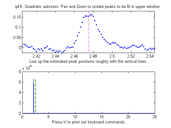
An easy way to do this is to use the interactive peak fitter ipf.m (described below) to explore various segments of the signal by panning and zooming and to try some trial fits and baseline correction settings, then press the "w" key to print out the peakfit syntax for that segment, with all its input arguments. Copy, paste, and edit the syntax for each segment as desired, then paste them into you code:
[FitResults1,
GOF1] = peakfit(datamatrix, center1, window1...
[FitResults2,
GOF2] = peakfit(datamatrix, center2, window2...
etc.
It is actually faster for the computer to execute a series of
smaller peakfit() commands like that than a single longer one
encompassing the entire data range in one go.
The
script FittingPeaksInMultiColumnData.m shows how to read a multi-column data set
from an Excel spreadsheet (BenzeneIR.xlsx)
and to use peakfit.m to fit a selected portion of the signal in
each column with a model consisting of 4 overlapping peaks. The
data, from the NIST InfraRed database, consists of 6 scans of
the gas-phase IR spectrum of benzene. The wavenumber axis is in
the first column of the spreadsheet and the 6 spectral scans are
in columns 2 through 7. Input arguments for the peakfit function
(lines 13-20) are based on previous exploration with the
interactive peak fitter (ipf.m,
below, left). The results for the best fit to each scan are
graphed (below, right), printed out in the command window, and
stored in the 4x5x6 matrix PP.


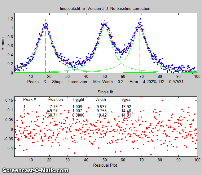
findpeaksfit.m
is essentially a combination of findpeaks.m
and peakfit.m. It
uses the number of peaks found and the peak positions and widths
determined by findpeaks as input for the peakfit.m function, which
then fits the entire signal with the specified peak model.
This combination function is more convenient that using findpeaks
and peakfit separately. It yields better values that findpeaks
alone, because peakfit fits the entire peak, not just the top
part, and because it deals with non-Gaussian and overlapped peaks.
However, it fits only those peaks that are found by findpeaks, so
you will have to make sure that every peak that contributes to
your signal is located by findpeaks. The syntax is
function [P,FitResults,LowestError,residuals,xi,yi] =
findpeaksfit(x, y, SlopeThreshold, AmpThreshold,
smoothwidth, peakgroup, smoothtype, peakshape, extra,
NumTrials, BaselineMode, fixedparameters, plots)
The first seven input arguments are exactly the same as for the findpeaks.m
function; if you have been using findpeaks or iPeak to find and
measure peaks in your signals, you can use those same input
argument values for findpeaksfit.m. The remaining six input
arguments of findpeaksfit.m are for the peakfit function; if you
have been using peakfit.m or ipf.m
to fit peaks in your signals, you can use those same input
argument values for findpeaksfit.m. Type "help findpeaksfit" for
more information. This function is included in the ipf13.zip distribution.
The animation on the right was created by the demo script findpeaksfitdemo.m. It shows
findpeaksfit finding and fitting the peaks in 150 signals, each of
which has 1 to 3 noisy Lorentzian peaks in variable locations.
The script FindpeaksComparison.m
compares the peak parameter accuracy of findpeaksG/L, findpeaksb,
findpeaksb3, and findpeaksfit applied to a
computer-generated signal with multiple peaks plus variable types
and amounts of baseline and random noise. The last three of these
functions include peak fitting equivalent to peakfit.m, in which
the number of peaks and the "first guess" starting values are
determined by findpeaksG/L.
 Matlab version of
the peak fitter for x,y data, which runs in Matlab on
your computer or in a Web
browser using Matlab
Online. (Octave versions can use the Octave version
ipfoctave.) and
uses keyboard commands and the mouse cursor. It is written
as a self- contained Matlab function, in a single m-file. The
flexible input syntax allows you to specify the data as separate
x,y vectors or as a 2xn matrix, and to optionally define the
initial focus by adding "center" and "window" values as
additional input arguments, where 'center' is the desired
x-value in the center of the upper window and "window" is the
desired width of that window. For example:
Matlab version of
the peak fitter for x,y data, which runs in Matlab on
your computer or in a Web
browser using Matlab
Online. (Octave versions can use the Octave version
ipfoctave.) and
uses keyboard commands and the mouse cursor. It is written
as a self- contained Matlab function, in a single m-file. The
flexible input syntax allows you to specify the data as separate
x,y vectors or as a 2xn matrix, and to optionally define the
initial focus by adding "center" and "window" values as
additional input arguments, where 'center' is the desired
x-value in the center of the upper window and "window" is the
desired width of that window. For example: ese m-files,
right-click on these links, select Save
Link As..., and click Save.
You can also download a ZIP file containing
ipf.m, Demoipf.m, and peakfit.m.
ese m-files,
right-click on these links, select Save
Link As..., and click Save.
You can also download a ZIP file containing
ipf.m, Demoipf.m, and peakfit.m.
(The function ShapeDemo demonstrates the basic peak shapes graphically, showing the variable-shape peaks as multiple lines)

Practical
examples with experimental data:
 1. Fitting weak and noisy peaks. In this example, pan and zoom controls are used to isolate a segment of a chromatogram that contains three very weak peaks near 5.8 minutes The lower plot shows the whole chromatogram and the upper plot shows the segment. Only the peaks in that segment are subjected to the fit. Pan and zoom are adjusted so that the signal returns to the local baseline at the ends of the segment. |
 Pressing T selects BaselineMode mode 1, causing the program to subtract a linear baseline from these data points. Pressing 3, E, F performs a 3-peak exponentially-broadened Gaussian fit (a common peak shape in chromatography). The A and Z keys are then used to adjust the time constant ("Extra") to obtain the best fit. The residuals (bottom panel) are random and exhibit no obvious structure, indicating that the fit is as good as is possible at this noise level. |
 The perpendicular drop method of
measuring the areas gives peak areas in a ratio of 25% and 75%,
compared to the actual 21% and 78% composition, which is not very
accurate probably because the peaks are visibly asymmetric. But an
exponentially-broadened Gaussian (a commonly-encountered peak shape
in chromatography) gives a fairly good fit to the data, using ipf.m
and adjusting the exponential term with the A and Z keys to get the
best fit. The results for a two-peak fit, shown in the ipf.m screen
on the right and in the R-key report below, show that the peak areas
are in a ratio of 23% and 77%, which is a bit better. With a 3-peak
fit, modeling the nitrogen peak as the sum of two closely
overlapping peaks whose areas are added together, the curve fit is much better (less than 1%
fitting error), and indeed the result in that case is 21.1% and
78.9% - considerably closer the the actual composition.
The perpendicular drop method of
measuring the areas gives peak areas in a ratio of 25% and 75%,
compared to the actual 21% and 78% composition, which is not very
accurate probably because the peaks are visibly asymmetric. But an
exponentially-broadened Gaussian (a commonly-encountered peak shape
in chromatography) gives a fairly good fit to the data, using ipf.m
and adjusting the exponential term with the A and Z keys to get the
best fit. The results for a two-peak fit, shown in the ipf.m screen
on the right and in the R-key report below, show that the peak areas
are in a ratio of 23% and 77%, which is a bit better. With a 3-peak
fit, modeling the nitrogen peak as the sum of two closely
overlapping peaks whose areas are added together, the curve fit is much better (less than 1%
fitting error), and indeed the result in that case is 21.1% and
78.9% - considerably closer the the actual composition. Percent Fitting
Error = 2.9318% Elapsed time = 11.5251 sec.
Peak# Position
Height Width Area
1 4.8385
17762 0.081094 1533.2
2 5.1439
47142 0.10205 5119.2
3. The accuracy of peak position measurement can be good even if
 the fitting error is rather poor. In this
example, an experimental high-resolution atomic emission spectrum is
examined in the region of the well-known
spectral lines of the element sodium. Two lines are found
there (figure on the right), and when fit to a unconstrained
Lorentzian or Gaussian model, the peak wavelengths are determined to
be 588.98 nm and 589.57 nm.
the fitting error is rather poor. In this
example, an experimental high-resolution atomic emission spectrum is
examined in the region of the well-known
spectral lines of the element sodium. Two lines are found
there (figure on the right), and when fit to a unconstrained
Lorentzian or Gaussian model, the peak wavelengths are determined to
be 588.98 nm and 589.57 nm. 
Peak Shape = Gaussian
Number of peaks = 3
Fitted range = 5 - 6.64
Percent Error = 7.4514 Elapsed time = 0.19741
Sec.
Peak# Position
Height
Width Area
1
5.33329
14.8274
0.262253 4.13361
2
5.80253
26.825
0.326065 9.31117
3
6.27707
22.1461
0.249248 5.87425
 |
 |
 Quadratic BaselineMode |

Note that, despite the noise in the data and the 8% fitting error, the bootstrap relative standard deviations are not so bad, especially for peak positions and heights. Notice that the RSD of the peak position is best (lowest), followed by height and width and area. This is a typical pattern, seen before. Also, be aware that the reliability of the computed variability depends on the assumption that the noise in the signal is representative of the average noise in repeated measurements. If the number of data points in the signal is small, these estimates can be very approximate.
If the RSD and the RSDIQR are roughly the same (as in the example above), then the distribution of bootstrap fitting results is close to normal and the fit is stable. If the RSD is substantially greater than RSD IQR, then the RSD is biased high by "outliers" (obliviously erroneous fits that fall far from the norm), and in that case you should use the RSD IQR rather than the RSD, because the IQR is much less influenced by outliers. (Alternatively, you could use another model or a different data set to see if that gives more stable fits).
A likely pitfall with the bootstrap method when applied to iterative fits is the possibility that one (or more) of the bootstrap fits will go astray, that is, will result in peak parameters that are wildly different from the norm, causing the estimated variability of the parameters to be too high. For that reason, in ipf 12.3 and later, two measures of uncertainty are calculated: (a) the regular standard deviation (STD) and (b) the standard deviation estimated by dividing the interquartile range (IQR) by 1.34896, which is labeled RSD (IQR). The IQR is more robust to outliers that STD. For a normal distribution, the interquartile range is on average equal to 1.34896 times the standard deviation. If one or more of the bootstrap sample fits fails, resulting in a distribution of peak parameters with large outliers, the regular STD will be much greater that the IQR. In that case, a more realistic estimate of variability is IRQ/1.34896. It's best to try to increase the fit stability by choosing a better model (e.g. using an equal-width or fixed-width model, or a fixed-position shape, if appropriate), adjusting the fitted range (pan and zoom keys), the background subtraction (T or B keys), or the start positions (C key), and/or selecting a higher number of fit trials per bootstrap (which will increase the computation time). As a quick preliminary test of bootstrap fit stability, pressing the N key will perform a single iterative fit to a random bootstrap sub-sample and plot the result; do that several times to see whether the bootstrap fits are stable enough to be worth computing a 100-sample bootstrap. Note: it's normal for the stability of the bootstrap sample fits (N key: click here for animation) to be poorer than the full-sample fits (F key; click here for animation), because the latter includes only the variability caused by changing the starting positions for one set of data and noise, whereas the N and V keys aim to include the variability caused by the random noise in the sample by fitting bootstrap sub-samples. Moreover, the best estimates of the measured peak parameters are those obtained by the normal fits of the full signal (F and X keys), not the means reported for the bootstrap samples (V and N keys), because there are more independent data points in the full fits and because the bootstrap means are influenced by the outliers that occur more commonly in the bootstrap fits. The bootstrap results are useful only for estimating the variability of the peak parameters, not for estimating their mean values. The N and V keys are also very useful way to determine if you are using too many peaks in your model; superfluous peaks will be very unstable when N is press repeatedly and will have much higher standard deviation of its peak height when the V key is used.
19. Shift-o fits a simple polynomial (linear, quadratic, cubic, etc) to the segment of the signal displayed in the upper panel and displays the polynomial coefficients (in descending powers) and the R2.
20. If some peaks are saturated and have a flat top (clipped at a maximum height), you can make the program ignore the saturated points by pressing Shift-M and entering the maximum Y values to keep. Y values above this limit will simply be ignored; peaks below this limit will be fit as usual.
21.
To constrain the model to peaks above a certain width, press Shift-W and enter the minimum peak with allowed.
a) The execution time can vary over a factor of 4 or 5 or more between different computers, (e.g. a small laptop with 1.6 GHz, dual core Athlon CPU with 4 Gbytes RAM, vs a desktop with a 3.4 GHz i7 CPU with 16 Gbytes RAM). Run the Matlab "bench.m" benchmark test to see how your computer stacks up.Other factors that are less important are the number of data points in the fitted region (but only if the number of data points is very large; for example see PeakfitTimeTest3.m) and the starting values (good starting values can reduce execution time slightly; PeakfitTimeTest2.m and PeakfitTimeTest2a.m have examples of that). Note: some of these scripts need DataMatrix2 and DataMatrix3, which you can download from http://tinyurl.com/cey8rwh.
b) The execution time increases with the product of the number of peaks in the model times the number of iterated variables per peak. (See PeakfitTimeTest.m).
c) The execution time varies greatly (sometimes by a factor of 100 or more) with the peak shape, with the exponentially-broadened shapes being the slowest and the fixed-width shapes being the fastest. See PeakfitTimeTest2.m and PeakfitTimeTest2a.m The equal-width and fixed-width shape variations are always faster.
d) The execution time increases directly with NumTrials in peakfit.m. The "Best of 10 trials" function (X key in ipf.m) takes about 10 times longer than a single fit.
Like the
other Live Scripts described above, PeakFittingTool.mlx
has a file browser button in line 1 and a pair of sliders in
lines 4 and 5 for setting the desired segment to work on. But
before opening a file, it's a good idea to temporarily de-select
the "FitPeaks" check-box in line 14, then when you have set all
the other controls, click it back on. That way you
will avoid waiting for unnecessary curve fit operations until
the appropriate settings are complete. (In challenging cases,
curve fitting operations can be slow and can take several
seconds in difficult cases).

Note: you can double-click
sliders to change their ranges if the initial range is
insufficient.
Note: to obtain the a digitally sampled
model, use peakfit's 6th and 7th output
parameters, xi and yi, which return a 600-point interpolated
model. Type plot(xi,yi) to plot each model peak separately or
plot(xi,yi(1,:)) to plot peak 1.
It's easier than you think to add your own custom peak shape to peakfit.m (or to those interactive functions that use peakfit.m, such as ipf.m, iSignal, or iPeak), assuming that you have a mathematical expression for your shape. The easiest way is to modify an existing peak shape that you do not plan to use, replacing it with your new function. Pick a shape to sacrifice that has the same number of variables and constraints are your new shape. For example, if your shape has two iterated parameters (e.g., variable position and width), you could modify the Gaussian, Lorentzian, or triangular shape (number 1, 2 or 21, respectively). If your shape has three iterated variables, use shapes like 31 (Shift-R), 32, 33, or 34. If your shape has four iterated variables, use shape 49 ("Pearson IV", Shift-K). If your shape has an 'extra' parameter, like the equal-shape Voigt, Pearson, BWF, or blended Gaussian/ Lorentzian, use one of those. If you need an exponentially modified shape, use the exponentially modified Gaussian (5 or 31) or Lorentzian (18). If you need equal widths or fixed widths, etc., use one of those shapes. This is important; you must have the same number of variables and constraints, because the structure of the code is different for each class of shapes.
There are just two required
steps to the process:
1. Let's say that your
shape has two iterated parameters and you are going to sacrifice
the triangular shape, number 21. Open peakfit.m or ipf.m in the
Matlab editor and re-write the old shape function ("triangular",
located near line 3672 in ipf.m - there is one of those
functions for each shape - by changing name of the function and
the mathematics of the assignment statement (e.g. g =
1-(1./wid).*abs(x-pos);). You can use the same variables
('x' for the independent variable, 'pos' for peak position,
'wid' for peak width, etc.) Scale your function to have a peak
height of 1.0 (e.g. after computing y as a function of x, divide
by max(y)).
2. Use the search function in Matlab to find all instances of
the name of the old function and replace it with the new name,
checking "Wrap around" but leaving "Match case" and "Whole word"
unchecked in the Search box. If you do it right, for example,
all instances of "triangular" and all instances of
"fittriangular' will be modified with your new name replacing
"triangular". Save the result (or Save as... with a modified
file name).
That's it! Your new shape will now be shape 21 (or whatever was
the shape number of the old shape you sacrificed). In ipf.m, it
will be activated by the same keystroke used by the old shape
(e.g. Shift-T for the triangular, key number 84), and in iSignal
and in iPeak, the menu of peak shapes will have been modified by
the search and replace in step 2.
If you wish, you can change the keystroke assignment in ipf.m; first, find a key or Shift-Key that is not yet assigned (and which gives an "UnassignedKey" error statement when you press it with ipf.m running). Then change the old key number 84 to that unassigned one in the big "switch double(key)," case statement near the beginning of the code. But it's simpler just to use the old key.
Last update, June, 2023 Number of unique visits since May 17, 2008: