The most basic signal processing functions are those that involve
simple signal arithmetic: point-by-point addition, subtraction,
multiplication, or division of two signals or of one signal and a
constant. Despite their mathematical simplicity, these functions
can be very useful. For example, in the left part of the figure
below, the top curve is the optical absorption spectrum of an
extract of a sample of oil shale, a kind of rock that is is a
source of petroleum.
A simple point-by-point subtraction of two signals
allows the background (bottom curve on the left) to be
subtracted from a complex sample (top curve on the left),
resulting in a clearer picture of what is really in the sample
(right). (X-axis = wavelength in nm; Y-axis = absorbance).
This optical spectrum exhibits
two absorption peaks, at about 515 nm and 550 nm, that are due
to a class of molecular fossils of chlorophyll called porphyrins.
(Porphyrins are used as geomarkers in oil exploration). These
absorption peaks are superimposed on a background absorption
caused by the extracting solvents and by non-porphyrin compounds
extracted from the shale. The bottom curve is the spectrum of an
extract of a non-porphyrin-bearing shale, showing only the
background absorption. To obtain the spectrum of the shale
extract without the background, the background (bottom curve) is
simply subtracted from the sample spectrum (top curve). The
difference is shown in the right in Window 2 (note the change in
Y-axis scale). In this case the removal of the background is not
perfect, because the background spectrum is measured on a
separate shale sample. However, it works well enough that the
two bands are now seen more clearly and it is easier to measure
precisely their absorbances and wavelengths. (Thanks to the late
Prof. David Freeman for the spectra of oil shale extracts).
In this example and the one
below, I am making the assumption that the two signals in Window
1 have the same x-axis values - in other words, that
both spectra are digitized at the same set of wavelengths.
Subtracting or dividing two spectra would not be valid if two
spectra were digitized over different wavelength ranges or with
different intervals between adjacent points. The x-axis values
must match up point for point. In practice, this is very often
the case with data sets acquired within one experiment on one
instrument, but the experimenter must be careful if the
instruments settings are changed or if data from two experiments
or two different instrument are combined. It is possible to use
the mathematical technique of interpolation to change
the number of points or to equalize unequally-spaced x-axis
intervals of signals; the results are only approximate but often
close enough in practice. Matlab and Octave has several built in
functions for linear and cubic spline interpolation; see the Matlab/Octave script CompareInterp1andSpline.m
(graphic on the
right) and CompareInterpolationMethods2.m
(graphic).
(Interpolation is one of the functions of my
multi-purpose interactive iSignal function described
later).
Sometimes one needs to know whether
two signals have the same shape, for example in comparing the
signal of an unknown to a stored reference signal. Most likely
the amplitudes of the two signals, will be different. Therefore
a direct overlay or subtraction of the two signals will not be
useful. One possibility is to compute the point-by-point ratio
of the two signals; if they have the same shape, the ratio will
be a constant. For example, examine Figure 2.
Do the two signals on the left have the same
shape? They certainly do not look the same, but that may
simply be due to the fact that one is much weaker than the
other. The ratio of the two signals, shown in the
right part (Window 2), is relatively constant from 300 to 440
nm, with a value of 10 +/- 0.2. This means that the shape of
these two signals is very nearly identical over this x-axis
range.
The left part (Window 1) shows two superimposed signals,
one of which is much weaker than the other. But do they have the
same shape? The ratio of the two signals, shown in the right
part (Window 2), is relatively constant from x=300 to 440, with
a value of 10 +/- 0.2. This means that the shape of these two
signals is the same, within about +/-2 %, over this x-axis
range, and that top curve is very nearly 10 times more intense
than the bottom one. Above x=440 the ratio is not even
approximately constant; this is caused by noise, which
is the subject of the next
section.
A division by zero error will be caused by even
a single zero in the denominator vector, but that can
usually be avoided by applying a small amount of
smoothing of the denominator, by
adding a small positive number to the vector, or by using the
custom Matlab/Octave function rmz.m (remove
zeros), which replaces zeros with the nearest non-zero
numbers, or the nlt.m (no lower
than) function that limits the lowest number in a vector
to a specified value.
On-linecalculations and
plotting.Wolfram
Alpha is a Web site and a smartphone app
that is a computational tool and information source, including
capabilities for mathematics,
plotting
data and functions, vector and matrix
manipulations, statistics
and data analysis, and many other topics. Statpages.org can
perform a huge range of statistical calculations and tests. There
are several Web sites that specialize in plotting data, including
Tableau, Plotly, Grapher, and Plotter. All of
these require a reliable Internet connection, and they can be
useful when you are working on a mobile device or a on computer
that does not have the required software.
Popular spreadsheets, such as Excelor Open Office Calc, have
built-in functions for all common math operations, named variables,
x,y plotting, text formatting, matrix math, etc. (For a list of
Excel functions with tutorials on how to use them, see
https://computeexpert.com/english-blog/excel-formulas-list.)
Spreadsheet cells can contain numerical values, text,
mathematical expression, or references to other cells. A vector of
values such as a spectrum can be represented as a row or
column of cells; a rectangular array of values such as a set
of spectra can be represented as a rectangular block of cells.
User-created names can be assigned to individual cells or to
ranges of cells, then referred to in mathematical expression by
name. Mathematical expressions can be easily copied across a range
of cells, with the cell references changing or not as desired.
Plots of various types (including the all-important x-y or
scatter graph) can be created by menu selection. See http://www.youtube.com/watch?v=nTlkkbQWpVk
for a nice video demonstration. Both Excel and Calc
offer a form design capability with full set of user interface
objects such as buttons, menus, sliders, and text boxes; these can
be user to create attractive graphical user interfaces for
end-user applications, such as in http://terpconnect.umd.edu/~toh/models/.
The latest versions of both Excel (Excel 2013) and OpenOffice Calc (3.4.1) can open and
save either spreadsheet file format (.xls and .ods, respectively).
Simple spreadsheets in either format are compatible with the other
program. However, there are small differences in the way that
certain functions are interpreted, and for that reason I supply
most of my spreadsheets in .xls (for Excel) and in .ods (for Calc) formats. See "Differences
between the OpenDocument Spreadsheet (.ods) format and the Excel
(.xlsx) format". Basically, Calc and do most everything Excel can do, but Calc is free to download and
is more Windows-standard in terms of look-and-feel. Excel is more
"Microsoft-y" and for some operations is faster than Calc.
If you have access to Excel, I would use that.
If you are working on a tablet or smartphone, you could use the
Excel
mobile app, Numbers
for iPad, or several other mobile
spreadsheets. These can do basic tasks but do not have the
fancier capabilities of the desktop computer versions. By saving
their data in the "cloud" (e.g. iCloud or SkyDrive), these apps
automatically sync changes in both directions between mobile
devices and desktop computers, making them useful for field data
entry. Matlab
is a "multi-paradigm numerical computing environment and
fourth-generation programming language" (Wikipedia). In
Matlab (and in Octave, its GNU clone), a
single variable can represent either a single "scalar" value, a vector of values (such as a
spectrum or a chromatogram), a matrix (a rectangular array of values, such as a
set of spectra), or a set of multiple matrices. All
the standard math operations and functions adjust to match.
This greatly facilitates mathematical operations on signal waveforms.
For example, if you have signal
amplitudes in the variable y,
you can plot it just by typing"plot(y)". And if you also have a vector tof the same length
containing the times at which each value of y was obtained, you can plot y vs t by typing "plot(t,y)". Two signals y
and z can be plotted on the same time axis for comparison
by typing "plot(t,y,t,z)" . (Matlab
automatically assigns different colors to each line, but you can
control the color and line style yourself by adding additional
symbols; for example "plot(y,y,'r.',y,z,'b-')"
will plot y with red dots and z with a blue
line. You can divide up one figure window into multiple
smaller plots by placing subplot(m,n,p) before the plot
command to plot in the pth section of a m-by-n grid of
plots. Here is a 2x2 example
of a subplot. Type "help plot" or "help subplot" for more options.
(Throughout this site, you can copy and paste, or drag and drop,
any of the single-line or multi-line code examples into the Matlab
or Octave editor or directly into the command line and press Enter
to execute it immediately).
For publication-quality graphs, click on a Figure window,
then click File > Export setup, choose the size,
resolution, color, fonts, etc, then click Export and
select the file format (e.g.TIF, eps, etc). You can also use PlotPub
, a downloadable library that is free, easy to use,
allows great flexibility in choosing graph details, and creates
great-looking graphs within Matlab that can be exported in EPS,
PDF, PNG and TIFF with adjustable resolution. Here's an example (script,
graphic).
The function max(y) returns the maximum value of
y and min(y) returns the minimum.
Individual elements in a vector are referred to by index
number; for example, t(10) is the 10th
element in vector t, and t(10:20) is the
vector of values of t from the 10th to the 20th entries.
You can find the index number of the entry closest to a given
value in a vector by using the downloadable val2ind.m
function; for example, t(val2ind(y,max(y)))
returns the time of the maximum y, and t(val2ind(t,550):val2ind(t,560))
is the vector of values of t between 550 and 560 (assuming
t contains values within that range). The units of
the time data in the t vector could be anything -
microseconds, milliseconds, hours, any time units.
A Matlab variable can also be a matrix, a set of vectors
of the same length combined into a rectangular array. For example,
intensity readings of 10 different optical spectra, each taken at
the same set of 100 wavelengths, could be combined into the 10x100
matrix S. S(3,:) would be the third of those
spectra and S(5,40) would be the intensity at the 40th
wavelength of the 5th spectrum. The Matlab/ Octave scripts plotting.m and plotting2.m show
how to plot multiple signals using matrices and subplots.
The subtraction of two signals a
and b, as in Figure 1, can be
performed simply by writing a-b.
To plot the difference, you would write "plot(a-b)". Likewise, to
plot the ratio of two signals, as in Figure 2, you would write "plot(a./b)". So, "./" means
divide point-by-point and ".*" means multiply point-by-point. The
* by itself means matrix multiplication, which you can use to
perform repeated multiplications without using loops. For example,
if x is a vector
A=[1:100]'*x;
creates a matrix A in which each column is x multiplied by
the the numbers 1, 2,...100. It is equivalent to, but more compact
and up to 300 times faster than, writing a
"for" loop like this:
for n=1:100; A(:,n)=n.*x; end;
Yes, that's right, it makes that much difference, at least in this
simple example. It will be faster if you pre-allocate memory space
for the A matrix by adding the statement A=zeros(100,100)
before the loop. But even then the matrix notation is faster than
the loop.
In Matlab/Octave, "/" is not the same as "\". Typing "b\a" will
compute the "matrix
right divide", in effect the weighted average ratio of the
amplitudes of the two vectors (a type of least-squares best-fit
solution), which in the example in Figure 2 will be a number close
to 10. The point here is that Matlab doesn't require you to
deal with vectors and matrices as collections of numbers; it
knows when you are dealing with matrices, or when the result of a
calculation will be a matrix, and it adjusts your calculations
accordingly. See http://www.mathworks.com/help/matlab/matlab_prog/array-vs-matrix-operations.html.
Probably the most common errors you'll make in Matlab/Octave are
punctuation errors, such as mixing up periods, commas, colons, and
semicolons, or parentheses, square brackets, and curly brackets;
type "help punct" at the Matlab
prompt and read the help file until you fall asleep. Little
things can mean a lot in Matlab. Another common error is
getting the rows and columns of vectors and matrices mixed up.
(Full disclosure: I still make all these kinds of
mistakes all the time). Here's a text
file that gives examples of common vector and matrix
operations and errors in Matlab and Octave. If you are new to
this, I recommend that you read this file and play around with the
examples there. Writing Matlab is a trial and error process, with
the emphasis on error.
There are many code examples in
this text that you can Copy and Paste and modify into the
Matlab/Octave command line, which is a great way to learn
and is especially convenient if you can position the windows so that
Matlab shares the screen with this website (e.g. Matlab on the
left and web browser on the right (click
for graphic) or (even better) if you
have two monitors hooked to your computer configured to expand
the desktop horizontally.If you try
to run one of my scripts or functions and it gives you a
"missing function" error, look for the missing item on functions.html, download
it into your path, and try again.
Matlab
Compiler is a separately available product that lets you
share programs as standalone applications, and Matlab
Compiler SDK lets you build C/C++ shared libraries,
Microsoft .NET assemblies, Java classes, and Python packages
from Matlab programs. Getting data into Matlab/Octave. You
can easily import
your own data into Matlab or Octave, for example by using
the xlsread or importdata
functions at the command line or in your own scripts. Data can be
imported from plain text files (.txt), CSV files (comma separated
values), from several image and sound formats, or from
spreadsheets. For example, the following lines will read the first
two columns of the csv file "Sample_5.0ppm.csv" in the
current folder and assign them to the vectors x and y. mydata=xlsread('Sample_5.0ppm.csv'); x=mydata(:,1); y=mydata(:,2);
The script "xlsreadDemo.m"
provides a simple
example of reading a multi-column spreadsheet “xlsx” file.
For more complex spreadsheets,
Matlab has a convenient Import Wizard (click File >
Import Data) that gives you a preview into the data file,
parses the data file looking for columns and rows of numeric data
and their labels, and gives you a chance to select and re-label
the desired variables and to choose the output type. You can even
click on the little arrow to the right of "Import selection" and Matlab
will write you a script that will perform those operations,
which you can modify for other file types and formats.
JCAMP-DX is a standard
file form for exchange of infrared spectra and related
chemical and physical information between spectrometer data
systems of different manufacture. Matlab’s jcampread function
can import such data. For an example, see ReadJcampExample.m.
It is also possible to import data from graphical line plots
or printed graphs by using the built-in "ginput" function
that obtains numerical data from the coordinates of mouse clicks
(as in
DataTheif or Figure
Digitizer).
Python
can import data in text, CSV, JSON, Matlab, and several
other formats, using the Variable Explorer panel in the Spyder
desktop, or through the separately downloadable Pandas Data Analysis
package.
Matlab Versions. The standard commercial version of Matlab is expensive (over $2000) but don't let
that frighten you - there are student and home versions that
cost muchless (as
little as $49 for a basic student version) and have all the
capabilities to perform any of the methods detailed in this book
at comparable execution
speeds. There is also Matlab
Online, which runs in a web browser (left); and
the free Matlab
Mobile app that runs
Matlab on iPads and even iPhones (right).
This requires only a basic student license and uses whatever
functions, scripts, and data that you have previously uploaded
to your free account on the Matlab cloud. Notably, all these versions have
computational speeds within roughly a factor of 2 of each other,
as shown by the text file TimeTrial.txt,
which lists measured execution speeds for for a variety of signal processing
tasks running on four different hardware/software
configurations: Matlab 2020b, Matlab Online,
R2018b, and Matlab Mobile (iPad). See https://www.mathworks.com/pricing-licensing.html. GNU Octave
is a free
alternative to Matlab that is "mostly
compatible"
.
DspGURU says
that Octave is "...a mature high-quality Matlab clone. It has the
highest degree of Matlab compatibility of all the clones."
Everything I said above about Matlab also works in Octave. In
fact, the most recent versions
of almost all of my Matlab functions, scripts, demos,
and examples in this document will work in the latest version of
Octave without change. (The keystroke-operated
interactive functions requires separate Octave versions
ipeakoctave.m, isignaloctave.m, and ipfoctave.m). If you plan to
use Octave, make sure you get the current versions; many of them
were updated for Octave compatibility in 2015 and this is an
ongoing project. There is a FAQ that may help in porting
Matlab programs to Octave. See Key
Differences Between Octave & Matlab. There are Windows,
Mac, and Unix versions of Octave; the Windows version can be
downloaded from Octave
Forge; be sure to install all the "packages". There is lots
of help online: Google "GNU
Octave" or see the YouTube
videos for help. For signal processing applications
specifically, Google "signal
processing octave".
Note: the older Octave 3.6 can even run
on a Raspberry Pi (a low-cost
single-board computer).
Octave Version 6.4.0 has been
released and is now available fordownload.
It is much improved over older previous versions. New versions
are introduced often. However, Octave is still computationally
about 6 times slower on average than the latest Matlab version,
depending on the task (for some specific
examples, see TimeTrial.txt). Bottom line: Matlab is better, but
if you can't afford Matlab, Octave provides almost all of the
functionality for 0% of the cost. Python, a scripted language that is a free open-source
alternative to Matlab, can be configured with almost all of the
capabilities of Matlab for scientific signal processing. See https://terpconnect.umd.edu/~toh/spectrum/Python.html Spreadsheet
or Matlab/Octave/Python? For signal processing,
Matlab/Octave and Python are faster and more powerful than using a
spreadsheet, but it's safe to say that spreadsheets are more
commonly installed on science workers' computers than Matlab or
Python. For one thing, spreadsheets are easier to get started with
and they offer flexible presentation and user interface design.
Spreadsheets are better for data entry and are easily deployed on
portable devices such as smartphones and tablets (e.g. using iCloud Numbers
or the Excel
app). Spreadsheets are concrete and more low-level,
showing every single value explicitly in a cell. Matlab/Octave
is more high level and abstract, because a single variable,
punctuation, or function can do so much. An advantage of Matlab and Octave
is that their function and script files ("m-files") are just
plan text files with a ".m" extension, or ".py" in Python, so
those files can be opened and inspected using any text
editor, even on devices that do not have those programs
installed. Also, user-defined
functions can call other built-in or user-defined functions, which
in turn can call other functions, and so on, allowing very
complex high-level functions to be built up in layers.
Fortunately, Matlab can easily read Excel .xls and .xlsx files and
import the rows and columns into matrix variables.
Using the analogy of electronic
circuits, spreadsheets are like old-school discrete component
electronics, where every resistor, capacitor, and transistor is a
discrete, macroscopic entity that you can see and manipulate
directly. A function-based programming language like Matlab/Octave
is more like micro-electronics, where the functions (the "m-files"
that begin with "function...") are the integrated circuit "chips",
that condense complex operations into one package with documented
input and output pins (the function's input and output arguments)
that you can connect to other functions, but which hide the
internal details (unless you care to look at the code, which you
always can do). A good example is the ubiquitous "555 timer", an
8-pin timer, pulse generator, and oscillator chip introduced in
1972, which has since become the most popular
integrated circuit ever manufactured. These days, almost all
electronics is done with chips of one type or another, because
it's easier to understand the relatively small number of inputs
and outputs of a chip than to deal with the greater number of
internal components.
Much of Matlab/Octave is actually written in the Matlab/Octave
language, using more basic functions to build more complex ones.
You can write new functions of your own that essentially extend
the language in whatever direction you need. Just remember to
include your custom functions whenever you share you code with
others.
The bottom line is that spreadsheets are easier at
first, but in my experience, sooner or later, writing in
Matlab/Octave/Python
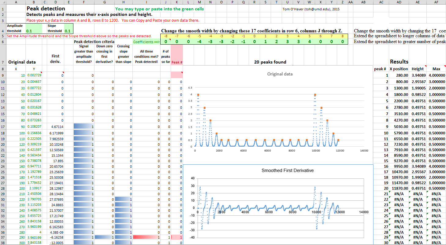
is more productive. This point is demonstrated by the
comparison of both platforms multilinear regression in
multicomponent spectroscopy (RegressionDemo.xls
vs the Matlab/Octave CLS.m), and particularly
by the dramatic difference between the spreadsheet
and Matlab/Octave
approaches to finding and measuring peaks in signals (i.e. a 250Kbyte spreadsheet
vs a 7Kbyte script that's 50 times
faster). If you have lots of data and you need to run it
through a multi-step customized process automatically,
hands-off, and as quickly as possible, then Matlab or Python is a
great way to go. It's much easier to write a script that
will automate the hands-off processing of volumes of data stored
in separate data files on your computer; an example is given in Appendix X.
Both spreadsheets and scripted language programs have a huge
advantage over commercial end-user programs and compiled freeware
programs such as SPECTRUM; the scripts and functions can be inspected
and modified by the user to customize the routines for
specific needs. Simple changes are easy to make with little or
little knowledge of programming. For example, you could easily
change the labels, titles, colors, or line style of the graphs -
in Matlab or Octave programs, search for "title(", "label(" or
"plot(". My code often contains comments that indicate places
where specific changes can easily be made: just use Find...
to search for the word "change". You are invited to modify my
scripts and functions as you wish.
Hint: This site contains many links to code and data examples,
Matlab/Octave scripts, enlarged graphics, screen images, and
spreadsheet templates; to view these alongside the text,
right-click and select "Open link in new window".
This page is part of "A Pragmatic
Introduction to Signal Processing", created and
maintained by Prof. Tom
O'Haver , Department of Chemistry and Biochemistry, The
University of Maryland at College Park. Comments, suggestions and
questions should be directed to Prof. O'Haver at toh@umd.edu.
Updated June, 2022.
 Window
1 have the same x-axis values - in other words, that
both spectra are digitized at the same set of wavelengths.
Subtracting or dividing two spectra would not be valid if two
spectra were digitized over different wavelength ranges or with
different intervals between adjacent points. The x-axis values
must match up point for point. In practice, this is very often
the case with data sets acquired within one experiment on one
instrument, but the experimenter must be careful if the
instruments settings are changed or if data from two experiments
or two different instrument are combined. It is possible to use
the mathematical technique of interpolation to change
the number of points or to equalize unequally-spaced x-axis
intervals of signals; the results are only approximate but often
close enough in practice. Matlab and Octave has several built in
functions for linear and cubic spline interpolation; see the Matlab/Octave script CompareInterp1andSpline.m
(graphic on the
right) and CompareInterpolationMethods2.m
(graphic).
(Interpolation is one of the functions of my
multi-purpose interactive iSignal function described
later).
Window
1 have the same x-axis values - in other words, that
both spectra are digitized at the same set of wavelengths.
Subtracting or dividing two spectra would not be valid if two
spectra were digitized over different wavelength ranges or with
different intervals between adjacent points. The x-axis values
must match up point for point. In practice, this is very often
the case with data sets acquired within one experiment on one
instrument, but the experimenter must be careful if the
instruments settings are changed or if data from two experiments
or two different instrument are combined. It is possible to use
the mathematical technique of interpolation to change
the number of points or to equalize unequally-spaced x-axis
intervals of signals; the results are only approximate but often
close enough in practice. Matlab and Octave has several built in
functions for linear and cubic spline interpolation; see the Matlab/Octave script CompareInterp1andSpline.m
(graphic on the
right) and CompareInterpolationMethods2.m
(graphic).
(Interpolation is one of the functions of my
multi-purpose interactive iSignal function described
later).

 math operations, named variables,
x,y plotting, text formatting, matrix math, etc. (For a list of
Excel functions with tutorials on how to use them, see
https://computeexpert.com/english-blog/excel-formulas-list.)
Spreadsheet cells can contain numerical values, text,
mathematical expression, or references to other cells. A vector of
values such as a spectrum can be represented as a row or
column of cells; a rectangular array of values such as a set
of spectra can be represented as a rectangular block of cells.
User-created names can be assigned to individual cells or to
ranges of cells, then referred to in mathematical expression by
name. Mathematical expressions can be easily copied across a range
of cells, with the cell references changing or not as desired.
Plots of various types (including the all-important x-y or
scatter graph) can be created by menu selection. See http://www.youtube.com/watch?v=nTlkkbQWpVk
for a nice video demonstration. Both Excel and Calc
offer a form design capability with full set of user interface
objects such as buttons, menus, sliders, and text boxes; these can
be user to create attractive graphical user interfaces for
end-user applications, such as in http://terpconnect.umd.edu/~toh/models/.
The latest versions of both Excel (Excel 2013) and OpenOffice Calc (3.4.1) can open and
save either spreadsheet file format (.xls and .ods, respectively).
Simple spreadsheets in either format are compatible with the other
program. However, there are small differences in the way that
certain functions are interpreted, and for that reason I supply
most of my spreadsheets in .xls (for Excel) and in .ods (for Calc) formats. See "Differences
between the OpenDocument Spreadsheet (.ods) format and the Excel
(.xlsx) format". Basically, Calc and do most everything Excel can do, but Calc is free to download and
is more Windows-standard in terms of look-and-feel. Excel is more
"Microsoft-y" and for some operations is faster than Calc.
If you have access to Excel, I would use that.
math operations, named variables,
x,y plotting, text formatting, matrix math, etc. (For a list of
Excel functions with tutorials on how to use them, see
https://computeexpert.com/english-blog/excel-formulas-list.)
Spreadsheet cells can contain numerical values, text,
mathematical expression, or references to other cells. A vector of
values such as a spectrum can be represented as a row or
column of cells; a rectangular array of values such as a set
of spectra can be represented as a rectangular block of cells.
User-created names can be assigned to individual cells or to
ranges of cells, then referred to in mathematical expression by
name. Mathematical expressions can be easily copied across a range
of cells, with the cell references changing or not as desired.
Plots of various types (including the all-important x-y or
scatter graph) can be created by menu selection. See http://www.youtube.com/watch?v=nTlkkbQWpVk
for a nice video demonstration. Both Excel and Calc
offer a form design capability with full set of user interface
objects such as buttons, menus, sliders, and text boxes; these can
be user to create attractive graphical user interfaces for
end-user applications, such as in http://terpconnect.umd.edu/~toh/models/.
The latest versions of both Excel (Excel 2013) and OpenOffice Calc (3.4.1) can open and
save either spreadsheet file format (.xls and .ods, respectively).
Simple spreadsheets in either format are compatible with the other
program. However, there are small differences in the way that
certain functions are interpreted, and for that reason I supply
most of my spreadsheets in .xls (for Excel) and in .ods (for Calc) formats. See "Differences
between the OpenDocument Spreadsheet (.ods) format and the Excel
(.xlsx) format". Basically, Calc and do most everything Excel can do, but Calc is free to download and
is more Windows-standard in terms of look-and-feel. Excel is more
"Microsoft-y" and for some operations is faster than Calc.
If you have access to Excel, I would use that. For example, if you have signal
amplitudes in the variable y,
you can plot it just by typing "plot(y)". And if you also have a vector t of the same length
containing the times at which each value of y was obtained, you can plot y vs t by typing "plot(t,y)". Two signals y
and z can be plotted on the same time axis for comparison
by typing "plot(t,y,t,z)" . (Matlab
automatically assigns different colors to each line, but you can
control the color and line style yourself by adding additional
symbols; for example "plot(y,y,'r.',y,z,'b-')"
will plot y with red dots and z with a blue
line. You can divide up one figure window into multiple
smaller plots by placing subplot(m,n,p) before the plot
command to plot in the pth section of a m-by-n grid of
plots. Here is a 2x2 example
of a subplot. Type "help plot" or "help subplot" for more options.
(Throughout this site, you can copy and paste, or drag and drop,
any of the single-line or multi-line code examples into the Matlab
or Octave editor or directly into the command line and press Enter
to execute it immediately).
For example, if you have signal
amplitudes in the variable y,
you can plot it just by typing "plot(y)". And if you also have a vector t of the same length
containing the times at which each value of y was obtained, you can plot y vs t by typing "plot(t,y)". Two signals y
and z can be plotted on the same time axis for comparison
by typing "plot(t,y,t,z)" . (Matlab
automatically assigns different colors to each line, but you can
control the color and line style yourself by adding additional
symbols; for example "plot(y,y,'r.',y,z,'b-')"
will plot y with red dots and z with a blue
line. You can divide up one figure window into multiple
smaller plots by placing subplot(m,n,p) before the plot
command to plot in the pth section of a m-by-n grid of
plots. Here is a 2x2 example
of a subplot. Type "help plot" or "help subplot" for more options.
(Throughout this site, you can copy and paste, or drag and drop,
any of the single-line or multi-line code examples into the Matlab
or Octave editor or directly into the command line and press Enter
to execute it immediately). 
 The standard commercial
  version of Matlab is expensive (over $2000) but don't let
that frighten you - there are student and home versions that
cost much less (as
little as $49 for a basic student version) and have all the
capabilities to perform any of the methods detailed in this book
at comparable execution
speeds. There is also Matlab
Online, which runs in a web browser (left); and
the free Matlab
Mobile app that runs
Matlab on iPads and even iPhones (right).
This requires only a basic student license and uses whatever
functions, scripts, and data that you have previously uploaded
to your free account on the Matlab cloud. Notably, all these versions have
computational speeds within roughly a factor of 2 of each other,
as shown by the text file TimeTrial.txt,
which lists measured execution speeds for for a variety of signal processing
tasks running on four different hardware/software
configurations: Matlab 2020b, Matlab Online,
R2018b, and Matlab Mobile (iPad). See https://www.mathworks.com/pricing-licensing.html.
version of Matlab is expensive (over $2000) but don't let
that frighten you - there are student and home versions that
cost much less (as
little as $49 for a basic student version) and have all the
capabilities to perform any of the methods detailed in this book
at comparable execution
speeds. There is also Matlab
Online, which runs in a web browser (left); and
the free Matlab
Mobile app that runs
Matlab on iPads and even iPhones (right).
This requires only a basic student license and uses whatever
functions, scripts, and data that you have previously uploaded
to your free account on the Matlab cloud. Notably, all these versions have
computational speeds within roughly a factor of 2 of each other,
as shown by the text file TimeTrial.txt,
which lists measured execution speeds for for a variety of signal processing
tasks running on four different hardware/software
configurations: Matlab 2020b, Matlab Online,
R2018b, and Matlab Mobile (iPad). See https://www.mathworks.com/pricing-licensing.html. Matlab functions, scripts, demos,
and examples in this document will work in the latest version of
Octave without change. (The keystroke-operated
interactive functions requires separate Octave versions
ipeakoctave.m, isignaloctave.m, and ipfoctave.m). If you plan to
use Octave, make sure you get the current versions; many of them
were updated for Octave compatibility in 2015 and this is an
ongoing project. There is a FAQ that may help in porting
Matlab programs to Octave. See Key
Differences Between Octave & Matlab. There are Windows,
Mac, and Unix versions of Octave; the Windows version can be
downloaded from Octave
Forge; be sure to install all the "packages". There is lots
of help online: Google "GNU
Octave" or see the YouTube
videos for help. For signal processing applications
specifically, Google "signal
processing octave".
Note: the older Octave 3.6 can even run
on a Raspberry Pi (a low-cost
single-board computer).
Matlab functions, scripts, demos,
and examples in this document will work in the latest version of
Octave without change. (The keystroke-operated
interactive functions requires separate Octave versions
ipeakoctave.m, isignaloctave.m, and ipfoctave.m). If you plan to
use Octave, make sure you get the current versions; many of them
were updated for Octave compatibility in 2015 and this is an
ongoing project. There is a FAQ that may help in porting
Matlab programs to Octave. See Key
Differences Between Octave & Matlab. There are Windows,
Mac, and Unix versions of Octave; the Windows version can be
downloaded from Octave
Forge; be sure to install all the "packages". There is lots
of help online: Google "GNU
Octave" or see the YouTube
videos for help. For signal processing applications
specifically, Google "signal
processing octave".
Note: the older Octave 3.6 can even run
on a Raspberry Pi (a low-cost
single-board computer).