Curve fitting A: Linear Least Squares

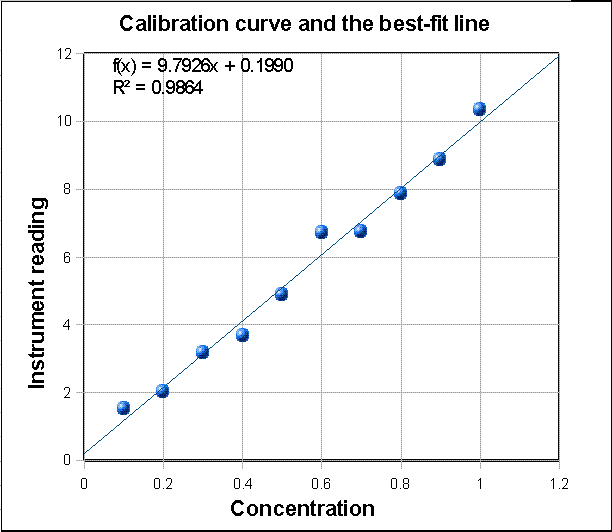
The graph on the left shows a third example, taken from analytical chemistry: a straight-line calibration data set where X = concentration and Y = instrument reading (Y = a + bX). Click to download that data. The blue dots are the data points. They don't all fall in a perfect straight line because of random noise and measurement error in the instrument readings and possibly also volumetric errors in the concentrations of the standards (which are usually prepared in the laboratory by diluting a stock solution). For this set of data, the measured slope is 9.7926 and the intercept is 0.199. In analytical chemistry, the slope of the calibration curve is often called the "sensitivity". The intercept indicates the instrument reading that would be expected if the concnetration were zero. Ordinarily instruments are adjusted ("zeroed") by the operator to give a reading of zero for a concentration of zero, but random noise and instrument drift can cause the intercept to be non-zero for any particular calibration set. In this computer-generated example, the "true" value of the slope was exactly 10 and of the intercept was exactly zero before noise was added, and the noise was added by a normally-distributed random-number generator, so the presence of the noise caused this particular measurement of slope to be off by about 2%. Had there been a larger number of points in this data set, the calculated values of slope and intercept would almost certainly have been better. (On average, the accuracy of measurements of slope and intercept improve with the square root of the number of points in the data set).

Once the calibration curve is established, it can be used to determine the conceentrations of unknown samples that are measured on the same instrument, for example by solving the equation for concentration as a function of instrument reading. The result is that the concentration of the sample Cx is given by Cx = (Sx-intercept)/slope, where Sx is the signal given by the sample solution, and "slope" and "intercept" are the results of the least-squares fit. The concentration and the instrument readings can be recorded in any convenient units, as long as the same units are used for calibration and for the measurement of unknowns.

 A plot of the "residuals" for the calibration data shows results that don't seem to be particularly random. Except for the the 6^th data point (at a concentration of 0.6), the other points seem to form a rough U-shaped curve, indicating that a quadratic or cubic equation might be a better model for those points. Can we reject the 6th point as being an "outlier", perhaps caused by a mistake in preparing that solution standard or in reading the instrument for that point?  The only way to know for sure is to repeat that standard solution preparation and calibration. Many instruments do give a very linear calibration response, but others show a slightly non-linear response under certain circumstances. In this particular case, the calibration data used for this example were computer-generated to be perfectly linear, with random numbers added to simulated noise.  So in fact that 6^th point is not an outlier and the curve is not non-linear, but you would not know that in a real application. Moral: don't throw out data points just because they seem a little off, unless you have good reason, and don't use higher-order polynomial fits just to get better fits if the instrument is known to give linear response under those circumstances. Even normally-distributed random errors can occasionally give individual deviations that are quite far from the average.

Reliability of  curve fitting results

How reliable are the slope, intercept and other polynomial coefficients obtained from least-squares calculations on experimental data? The single most important factor is the appropriateness of the model chosen; it's critical that the model (e.g. linear, quadratic, etc) be a good match to the actual underlying shape of the data. You can do that either by choosing a model based on the known and expected behavior of that system (like using a linear calibration model for an instrument that is known to give linear response under those conditions) or by choosing a model that always gives randomly-scattered residuals that do not exhibit a regular shape. But even with a perfect model, the least-squares procedure applied to repetitive sets of measurements will not give the same results every time because of random error (noise) in the data. If you were to repeat the entire set of measurements many times and do least-squares calculations on each data set, the standard deviations of the coefficients would vary directly with the standard deviation of the noise and inversely with the square root of the number of data points in each fit, all else being equal. The problem, obviously, is that it is not always possible to repeat the entire set of measurements many times. You may have only one set of measurements, and each experiment may be very expensive to repeat. So, we would like is some sort of short-cut method that would let us predict the standard deviations of the coefficients from a single measurement of the signal, without actually repeating the measurements.

Here I will describe three general ways to predict the standard deviations of the polynomial coefficients: algebraic propagation of errors, Monte Carlo simulation, and the bootstrap sampling method.

Algebraic Propagation of errors. The classical way is based on the rules for mathematical error propagation. The propagation of errors of the entire curve-fitting method can be described in closed-form algebra by breaking down the method into a series of simple differences, sums, products, and ratios, and applying the rules for error propagation to each step. The result of this procedure for a first-order (straight line) least-squares fit are shown in the last two lines of the set of equations in Math Details, below. Essentially, these equations make use of the deviations from the least-squares line (the "residuals") to estimate the standard deviations of the slope and intercept, based on the assumption that the noise in that single data set is representative of the noise that would be obtained upon repeated measurements. Because these predictions are based only on a single data set, they are good only insofar as that data set is typical of others that might be obtained in repeated measurements. If your random errors happen to be small when you acquire your data set, you'll get a deceptively good-looking fit, but then your estimates of the standard deviation of the slope and intercept will be too low, on average. If your random errors happen to be large in that data set, you'll get a deceptively bad-looking fit, but then your estimates of the standard deviation will be too high, on average. This problem becomes worse when the number of data points is small. This is not to say that it is not worth the trouble to calculate the predicted standard deviations of slope and intercept, but keep in mind that these predictions are accurate only if the number of data points is large (and only if the noise is random and normally distributed).  

In the application to analytical calibration, the concentration of the sample Cx is given by Cx = (Sx-intercept)/slope, where Sx is the signal given by the sample solution. The uncertainty of all three terms contribute to the uncertainty of Cx. The standard deviation of Cx can be calculated from the standard deviations of slope, intercept, and Sx using the rules for mathematical error propagation. But the problem is that, in analytical chemistry, the labor and cost of preparing and running large numbers of standards solution often limits the number of standards to a rather small set, by statistical standards, so these estimates of standard deviation are often fairly rough. (For a discussion and some examples, see http://terpconnect.umd.edu/~toh/models/Bracket.html#Cal_curve_linear. A spreadsheet that performs these error-propagation calculations for your own first-order analytical calibration data can be downloaded at http://terpconnect.umd.edu/~toh/models/CalibrationLinear2.ods).    

Monte Carlo simulation. The second way of estimating the standard deviations of the least-squares coefficients is to perform a random-number simulation (a type of Monte Carlo simulation). This requires that you know (by previous measurements) the average standard deviation of the random noise in the data. Using a computer, you construct a model of your data over the normal range of X and Y values (e.g. Y = intercept + slope*X + noise, where noise is the n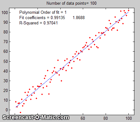oise in the data), compute the slope and intercept of each simulated noisy data set, then repeat that process many times (usually a few thousand) with different sets of random noise, and finally compute the standard deviation of all the resulting slopes and intercepts. This is ordinarily done with normally-distributed random noise (e.g. the RANDN function that many programing languages have). These random number genereators produce "white: noise.  If the model is good and the noise is white and well-characterized, the results will be a very good estimate of the expected standard deviations of the least-squares coefficients. (If the noise is not constant, but rather varies with the X or Y values, or if the noise is not white, then that must be included in the simulation). Obviously this method requires a computer and is not so convenient as evaluating a simple algebraic expression. But there are two important advantages to this method: (1) is has great generality; it can be applied to curve fitting methods that are too complicated for the classical closed-form algebraic propagation-of-error calculations, even iterative non-linear methods; and (2) its predictions are based on the average noise in the data, not the noise in just a single data set. For that reason, it gives more reliable estimations, particularly when the number of data points in each data set is small. Nevertheless, you can not always apply this method because you don't always know the average standard deviation of the random noise in the data.

You can download a MatlabOctave script that compares the Monte Carlo simulation to the algebraic method above from http://terpconnect.umd.edu/~toh/spectrum/LinearFiMC.m.  By running this script with different sizes of datasets ("NumPoints" in line 10), you can see that the standard deviation predicted by the algebraic method fluctuates a lot from run to run when NumPoints is small (e.g. 10), but the Monte Carlo predictions are much more steady.  When NumPoints is large (e.g. 1000), both methods agree very well.  

The Bootstrap. The third method is the "bootstrap" method, a procedure that involves choosing random subsamples with replacement from a single data set and analyzing each sample the same way (e.g. by a least-squares fit). Every sample is returned to the data set after sampling, so that (a) a particular data point from the original data set could appear multiple times in a given sample, and (b) the number of elements in each bootstrap subsample equals the number of elements in the original data set. As a simple examp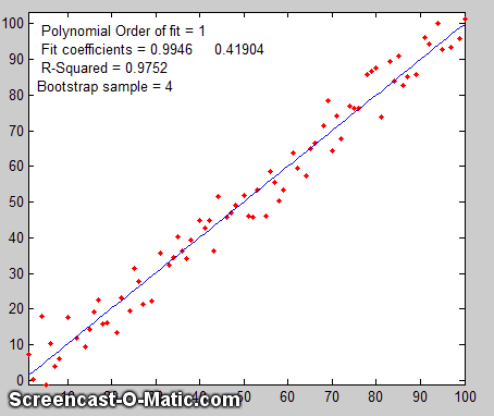le, consider a data set with 10 x,y pairs assigned the letters a through j. The original data set is represented as [a b c d e f g h i j], and some typical bootstrap subsamples might be [a b b d e f f h i i] or [a a c c e f g g i j], each bootstrap sample containing the same number of data points, but with about half of the data pairs skipped and the others duplicated. You would use a computer to generate hundreds or thousands of bootstrap samples like that and to apply the calculation procedure under investigation (in this case a linear least-squares) to each set. If there were no noise in the data set, and if the model were properly chosen, then all the points in the original data set and in all the bootstrap subsamples would fall exactly on the model line, and the least-squares results would be the same for every subsample. But if there is noise in the data set, each set would give a slightly different result (e.g. the least-squares polynomial coefficients), because each subsample has a different subset of the random noise. The greater the amount of random noise in the data set, the greater would be the range of results from sample in the bootstrap set. This enables you to estimate the uncertainty of the quantity you are estimating, just as in the Monte-Carlo method above. The difference is that the Monte-Carlo method is based on the assumption that the noise is known, random, normally-distributed, and can be accurately simulated by a random-number generator on a computer, whereas the bootstrap method uses the actual noise in the data set at hand, like the algebraic method, except that it does not need an algebraic solution of error propagation. The bootstrap method thus shares its generality with the Monte Carlo approach, but is limited by the assumption that the noise in that (possibly small) single data set is representative of the noise that would be obtained upon repeated measurements. This method is examined in detail in its extensive literature. 

The Matlab/Octave script TestLinearFit.m compares all three of these methods (Monte Carlo simulation, algebraic method, and the bootstrap method) for a 100-point first-order linear least-squares fit was performed. Each method is repeated on different data sets with the same average slope, intercept, and random noise, then the standard deviation (SD) of the slopes (SDslope) and intercepts (SDint)  were compiled and are tabulated below. 

(You can download this script from http://terpconnect.umd.edu/~toh/spectrum/TestLinearFit.m). On average, the mean standard deviation ("Mean SD") of the three methods agree very well, but the algebraic and bootstrap methods fluctuate more that the Monte Carlo simulation each time this script is run, because they are based on the noise in one single 100-point data set, whereas the Monte Carlo simulation reports the average of many data sets. Of course, the algebraic method is simpler and faster to compute than the other methods. However, an algebraic propagation of errors solution is not always possible to obtain, whereas the Monte Carlo and bootstrap methods do not depend on an algebraic solution and can be applied readily to more complicated curve-fitting situations, such as non-linear iterative least squares, as will be seen later.  

It's very important that the noisy signal not be smoothed before the least-squares calculations, because doing so will not improve the reliability of the least-squares results, but it will cause both the algebraic propagation-of-errors and the bootstrap calculations to seriously underestimate the standard deviation of the least-squares results. You can demonstrate using the most recent version of the script TestLinearFit.m by setting SmoothWidth in line 10 to something higher than 1, which will smooth the data before the least-squares calculations. This has no significant effect on the actual standard deviation as calculated by the Monte Carlo method, but it does significantly reduce the predicted standard deviation calculated by the algebraic propagation-of-errors and (especially) the bootstrap method.  For similar reasons, if the noise is pink rather than white, the bootstrap error estimates will also be low.  

Transforming non-linear relationships

In some cases a fundamentally non-linear relationship can be transformed into a form that is amenable to polynomial curve fitting by means of a coordinate transformation (e.g. taking the log or the reciprocal of the data), and then least-squares method can be applied to the resulting linear equation. For example, the signal in the figure below is from a simulation of an exponential decay (X=time, Y=signal intensity) that has the mathematical form Y = a exp(bX), where a is the Y-value at X=0 and b is the decay constant. This is a fundamentally non-linear problem because Y is a non-linear function of the parameter b. However, by taking the natural log of both sides of the equation, we obtain ln(Y)=ln(a) + bX. In this equation, Y is a linear function of both parameters ln(a) and b, so it can be fit by the least squares method in order to estimate ln(a) and b, from which you get a by computing exp(ln(a)). In this particular example, the "true" values of the coefficients are a =1 and b = -0.9, but random noise has been added to each data point, with a standard deviation equal to 10% of the value of that data point, in order to simulate a typical experimental measurement in the laboratory. An estimate of the values of  ln(a) and b, given only the noisy data points, can be determined by least-squares curve fitting of ln(Y) vs X. 

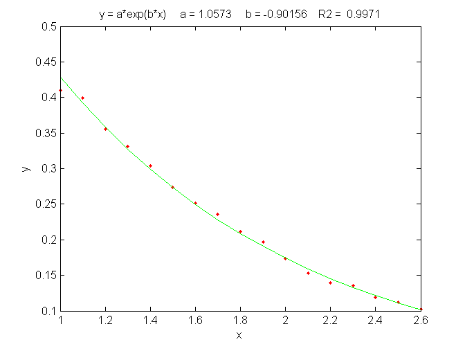
The best fit equation, shown by the green solid line in the figure, is Y =0.959 exp(- 0.905 X), that is, a = 0.959 and b = -0.905, which are reasonably close to the expected values of 1 and -0.9, respectively. Thus, even in the presence of substantial random noise (10% relative standard deviation), it is possible to get reasonable estimates of the parameters of the underlying equation (to within about 4%). The most important requirement is that the model be good, that is, that the equation selected for the model accurately describes the underlying behavior of the system (except for noise). Often that is the most difficult aspect, because the underlying models are not always known with certainty.  In Matlab and Octave, the fit can be performed in one line: polyfit(x,log(y),1), which returns [b log(a)]. (In Matlab and Octave, "log" is the natural log).

Other examples of non-linear relationships that can be linearized by coordinate transformation include the logarithmic (Y = a ln(bX)) and power (Y=aX^b) relationships. Methods of this type used to be very common back in the days before computers, when fitting anything but a straight line was difficult. It is still used today to extend the range of functional relationships that can be handled by common linear least-squares routines available in spreadsheets hand-held calculators.  (Only a few non-linear relationships can be handled this way, however. To fit any arbitrary custom function, you may have to resort to the more difficult non-linear iterative curve fitting method).

Fitting Peaks. An interesting example of the use of transformation to convert a non-linear relationship into a form that is amenable to polynomial curve fitting is the use of the natural log (ln) transformation to convert a Gaussian peak, which has the fundamental functional form exp(-x²), into a parabola of the form -x², which can be fit with a second order polynomial (quadratic) function (y = a + bx + cx²). The equation for a Gaussian peak is y = height*exp(-((x-position)./(0.6005615*width)) ^2), where height is the peak height, position is the x-axis location of the peak maximum, and width is the width of the peak at half-maximum. A little algebra will show that all three parameters of the peak (height, maximum position, and width) can be calculated from the three quadratic coefficients a, b, and c; the peak height is given by exp(a-c*(b/(2*c))^2), the peak position by -b/(2*c), and the peak half-width by 2.35482/(sqrt(2)*sqrt(-c)). (See Streamlining Digital Signal Processing: A Tricks of the Trade Guidebook, Richard G. Lyons, ed., page 298).  

An example is of this type of Gaussian curve fitting is shown in the figure on the left. The signal is a Gaussian peak with a true peak height of 100 units, a true peak position of 100 units, and a true half-width of 100 units, but it is sparsely sampled only every 31 units on the x-axis. The resulting data set, shown by the red points in the upper left, has only 6 data points on the peak itself.  If we were to take the maximum of those 6 points (the 3rd point from the left, with x=87, y=95) as the peak maximum, that would not be very close to the true values of peak position and height (100).  If we were to take the distance between the 2nd the 5th data points as the peak width, we'd get 3*31=93, again not very close to the true value of 100.  

However, taking the natural log of the data (upper right) produces a parabola that can be fit with a quadratic least-squares fit (shown by the blue line in the lower left). From the three coefficients of the quadratic fit we can calculate much more accurate values of the Gaussian peak parameters, shown at the bottom of the figure (height=100.57; position=98.96; width=99.2). The plot in the lower right shows the resulting Gaussian fit (in blue) displayed with the original data (red points). The accuracy of those peak parameters (about 1% in this example) is limited only by the noise in the data.  This above figure was created in Matlab (or Octave), using this script. The Matlab/Octave function gaussfit.m performs the calculation for an x,y data set. (You can also download a spreadsheet that fits a quadratic function to the natural log of y and computes the height, position, and width of the Gaussian that is a best fit to ln(y); it's available in OpenOffice Calc (Download link, Screen shot) and Excel formats.  Note: in order for this method to work properly, the data set must not contain any zeros or negative points; if the signal-to-noise ratio is very poor, it may be useful to pre-smooth the data slightly to prevent this problem. Moreover, the original Gaussian peak signal must be a single isolated peak with a zero baseline, that is, must tend to zero far from the peak center. In practice, this means that any non-zero baseline must be subtracted from the data set before applying this method.  A more general approch to fitting Gaussian peaks, which works for data sets with zeros and negative numbers and also for data with multiple overlapping peaks, is the non-linear iterative curve fitting method. 

A similar method can be derived for a Lorentzian peak, 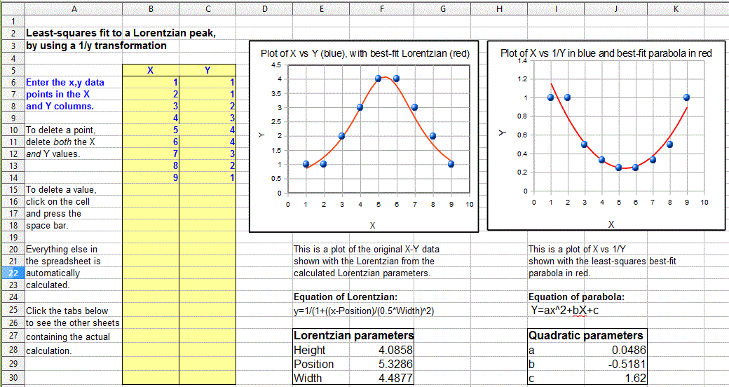which has the fundamental form 1/(1+x^2), by fitting a quadratic to the reciprocal of the y values. As for the Gaussian peak, all three parameters of the peak (height, maximum position, and width) can be calculated from the three quadratic coefficients a, b, and c of the quadratic fit. And just as for the Gaussian case, the data set must not contain any zeros or negative points. The Lorentzian peak height is given by 4*a./((4*a*c)-b^2), the peak position by -b/(2*a), and the peak half-width by sqrt(((4*a*c)-b^2)/a)/sqrt(a). The Matlab/Octave function lorentzfit.m performs the calculation for an x,y data set, and the Calc and Excel spreadsheets LorentzianLeastSquares.ods and LorentzianLeastSquares.xls perfrom the same calculation.  (By the way, a quick way to test either of the above methods is to use the simplest peak data set: x=1,2,3 and y=1,2,1, which has a height, width, and position all equal to 2, for a single peak of any shape, assuming a baseline of zero).

But there is a downside to using coordinate transformation methods to convert non-linear relationships into simple polynomial form, and that is that the noise is also effected by the transformation, with the result that the propagation of error from the original data to the final results is often difficult to predict. For example, in the method just described for measuring the peak height, position, and width of Gaussian or Lorentzian peaks, the results depends not only on the amplitude of noise in the signal, but also on how many points across the peak are taken for fitting. In particular, as you take more points far from the peak center, where the y-values approach zero, the natural log of those points approaches negative infinity as y approaches zero. The result is that the noise of those low-magnitude points is unduly magnified and has a disproportional effect on the curve fitting. This runs counter the usual expectation that the quality of the parameters derived from curve fitting improves with the square root of the number of data points (CurveFittingC.html#Noise).  A reasonable compromise in this case is to take only the points in the top half of the peak, with Y-values down to one-half of the peak maximum. If you do that, the error propagation (predicted by a Monte Carlo simulation with constant normally-distributed random noise) shows that the relative standard deviations of the measured peak parameters are directly proportional to the noise in the data and inversely proportional to the square root of the number of data points (as expected), but that the proportionality constants differ:

relative standard deviation of the peak height = 1.73*noise/sqrt(N),

relative standard deviation of the peak position = noise/sqrt(N), 

relative standard deviation of the peak width = 3.62*noise/sqrt(N), 

where noise is the standard deviation of the noise in the data and N in the number of data points taken for the least-squares fit. You can see from these results that the measurement of peak position is most precise, followed by the peak height, with the peak width being the least precise. If one were to include points far from the peak maxmum, where the signal-to-noise ratio is very low, the results would be poorer than predicted. These predictions depend on knowledge of the noise in the signal; if only a single sample of that noise is available for measurement, there is no guarantee that sample is a representative sample, especially if the total number of points in the measured signal is small; the standard deviation of small samples is notoriouly variable. Moreover, these predictions are based on a simulation with constant normally-distributed white noise; had the actual noise varied with signal level or with x-axis value, or if the probability distribution had been something other than normal, those predictions would not necessarily have been accurate. In such cases the bootstrap method has the advantage that it samples the actual noise in the signal. 

You can download the Matlab/Octave code for this Monte Carlo simulation from http://terpconnect.umd.edu/~toh/spectrum/GaussFitMC.m; view screen capture. A similar simulation (http://terpconnect.umd.edu/~toh/spectrum/GaussFitMC2.m, view screen capture) compares this method to fitting the entire Gaussian peak with the iterative method in Curve Fitting 3, finding that the precision of the results are only slightly better with the (slower) iterative method.   

Note 1: If you are reading this online, you can right-click on any of the m-file links above and select Save Link As... to download them to your computer for use within Matlab/Octave.

Note 2: In the curve fitting techniques described here and in the next two sections, there is no requirement that the x-axis interval between data points be uniform, as is the assumption in many of the other signal processing techniques previously covered.  Curve fitting algorithms typically accept a set of arbitrarily-spaced x-axis values and a corresponding set of y-axis values.

Math details.

The least-squares best fit for an x,y data set can be computed using only basic arithmetic.  Here are the relevant equations for computing the slope and intercept of the first-order best-fit equation, y = intercept + slope*x, as well as the predicted standard deviation of the slope and intercept, and the coefficient of determination, R², which is an indicator of the "goodness of fit". (R² is 1.0000 if the fit is perfect and less than that if the fit is imperfect).

(In these equations, Σ represents summation; for example, Σx means the sum of all the x values, and Σx*y means the sum of all the x*y products, etc).  The last two lines predict the standard deviation of the slope and intercept, based only on that data sample, assuming that the noise is normally distributed. These are estimates of the variability of slopes and intercepts you are likely to get if you repeated the data measurements over and over multiple times under the same conditions. Since the errors are random, they will be slightly different from time to time. The reliability of these standard deviation estimates depend on the number of data points in the curve fit; they improve with the square root of the number of points.

These calculations could be performed step-by-step by hand, with the aid of a calculator or a spreadsheet, with a program written in any programming language, or with a Matlab or Octave script. A similar set of equations can be written to fit a second-order (quadratic or parabolic) equations to a set of data.

You can also download spreadsheets in Excel and in OpenOffice Calc format (pictured above) that automate the computation of those equations and also plot the data and the best-fit line, requiring only that you type in (or paste in) the x-y data. There is one spreadsheet for linear fits (LeastSquares.xls and LeastSquares.odt) and also a version for quadratic (parabolic) fits (QuadraticLeastSquares.xls and QuadraticLeastSquares.ods).  

For the application to analytical calibration, there are specific versions of these spreadsheets that also calculate the concentrations of the unknowns.  There is also a set of spreadsheets that perform Monte Carlo simulations of widely-used analytical calibration methods, including typical systematic and random errors in both signal and in volumetric measurements, for the purpose of demonstrating how non-linearity, interferences, and random errors combine to influence the final result. 

It's important that the noisy signal (x.y) not be smoothed if the bootstrap error predictions are to be accurate. Smoothng the data will cause the bootstrap method to seriously underestimate the precision of the results.

Recent versions of Matlab have a convenient tool for interactive manually-controlled (rather than programmed) polynomial curve fitting in the Figure window. Click for a video example: (external link to YouTube).

The Matlab Statistics Toolbox includes two types of bootstrap functions, "bootstrp" and "jackknife".  To open the reference page in Matlab's help browser, type "doc bootstrp" or "doc jackknife".