
 Here's
how it works. The figure below shows, in Window 1, a
computer-generated peak (with a Lorentzian shape) in red,
superimposed on the negative of its second derivative in
green). (Click on the figure to see a full-size figure).
Here's
how it works. The figure below shows, in Window 1, a
computer-generated peak (with a Lorentzian shape) in red,
superimposed on the negative of its second derivative in
green). (Click on the figure to see a full-size figure). 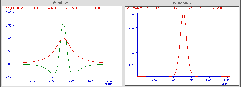
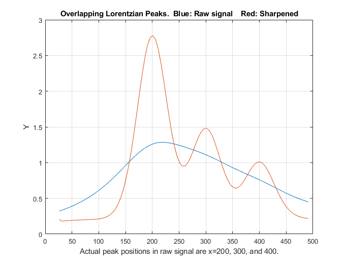 The reduced widths of
the sharpened peaks make it easier to distinguish overlapping peaks.
In the example on the right, the raw signal (blue line) is actually
composed of three overlapping Lorentzian peaks at x=200, 300, and
400, but the peaks are so wide - their halfwidths are 200, which is
greater than their separation - that they blend together in the raw
data, forming a wide asymmetrical peak with a maximum at x=220. The
result of derivative sharpening (red line) clearly shows the
underlying component peaks at their correct positions.
The reduced widths of
the sharpened peaks make it easier to distinguish overlapping peaks.
In the example on the right, the raw signal (blue line) is actually
composed of three overlapping Lorentzian peaks at x=200, 300, and
400, but the peaks are so wide - their halfwidths are 200, which is
greater than their separation - that they blend together in the raw
data, forming a wide asymmetrical peak with a maximum at x=220. The
result of derivative sharpening (red line) clearly shows the
underlying component peaks at their correct positions.  This
technique has been used in various forms of spectroscopy and
chromatography for many years (references
74-76), even in some cases using analog electronics.
Mathematically, the technique is a simplified version of a
converging Taylor
series expansion, in which only the even order
derivative terms in the expansion are taken and for which their
coefficients alternate in sign. The above example is the simplest
possible version that includes only the first two terms - the
original peak and its negative second derivative. Somewhat better
results can be obtained by adding a fourth derivative
term, with two adjustable factors k2 and k4:
This
technique has been used in various forms of spectroscopy and
chromatography for many years (references
74-76), even in some cases using analog electronics.
Mathematically, the technique is a simplified version of a
converging Taylor
series expansion, in which only the even order
derivative terms in the expansion are taken and for which their
coefficients alternate in sign. The above example is the simplest
possible version that includes only the first two terms - the
original peak and its negative second derivative. Somewhat better
results can be obtained by adding a fourth derivative
term, with two adjustable factors k2 and k4:
where Y'' and Y'''' are the 2nd and 4th derivatives of Y. The result is a 21% reduction in width for a Gaussian peak, as shown in the figure on the left (Matlab/Octave script), and a 60% reduction for a Lorentzian peak (script). This is the algorithm that was used in the overlapping peak example above. (It's possible to add a sixth derivative term, but the series converges quickly and the results are only slightly improved, at the cost of increased complexity of three adjustable factors).
There is no universal optimum value for the derivative weighting factors; it depends on what you consider the best trade-off between peak sharpening and baseline flatness. However, a good place to start for a Gaussian peak are k2 = W2/32 and k4 = W4/900, and for Lorentzian peaks, k2=W2/4 and k4 = W4/600, where W is the halfwidth (FWHM) of the peak before sharpening, in x units. With those weighting factors, a Gaussian peak will be reduced in width by 21% and the resulting peak will still fit a Gaussian model with a percent fitting error of less than 0.3% and an R2 of 0.9999 (that is, very nearly a perfect fit). For a Lorentzian original shape, the peak width is reduced by a factor of 3, but the resulting peak fits a Gaussian model with a larger percent fitting error of 1.15% and an R2 of 0.9966. Larger k values will result in a narrower peak, but the baseline on both side of the peak will exhibit a more pronounced negative undershoot. The software described below aids in the selection of the optimum degree of sharpening. Note that the K factors for the 2nd and 4th derivatives vary with the width raised to the 2nd and 4th power respectively, so they can vary over a very wide numerical range for peaks of different width. For this reason, if the peak widths vary substantially across the signal, it's possible to use segmented and gradient versions of this method so that the sharpening can be optimized for each region of the signal (see below). First derivative symmetrization.
The
even-derivative
technique described above works best for symmetrical peaks
shapes. If the peak is asymmetrical - that is, slopes
down faster on one side than the other - then the weighted
addition (or subtraction) of a first derivative term,
Y', may be helpful, because the first derivative of a peak is
antisymmetric (positive on one side and negative on the
other). This is also an old technique, having been used in
chromatography since at least 1965 (reference 74),
where it has been called "de-tailing". In fact, this
works perfectly for exponentially broadened peaks of any
shape (reference 70), for example
the "exponentially modified Gaussian" (EMG) shape. In the graphic example on
the right, the original peak (in blue) tails to the right, and its
first derivative, Y', (dotted yellow) has a positive lobe on the
left and a broader but smaller negative lobe on the right. When
the EMG is added to the weighted first derivative, the positive
lobe of the derivative reinforces the leading edge
and the negative lobe suppresses the trailing edge, resulting
in improved symmetry.
First derivative symmetrization.
The
even-derivative
technique described above works best for symmetrical peaks
shapes. If the peak is asymmetrical - that is, slopes
down faster on one side than the other - then the weighted
addition (or subtraction) of a first derivative term,
Y', may be helpful, because the first derivative of a peak is
antisymmetric (positive on one side and negative on the
other). This is also an old technique, having been used in
chromatography since at least 1965 (reference 74),
where it has been called "de-tailing". In fact, this
works perfectly for exponentially broadened peaks of any
shape (reference 70), for example
the "exponentially modified Gaussian" (EMG) shape. In the graphic example on
the right, the original peak (in blue) tails to the right, and its
first derivative, Y', (dotted yellow) has a positive lobe on the
left and a broader but smaller negative lobe on the right. When
the EMG is added to the weighted first derivative, the positive
lobe of the derivative reinforces the leading edge
and the negative lobe suppresses the trailing edge, resulting
in improved symmetry.
 power n greater
than 1 (reference 61, 63). The effect of this is to change
the peak shapes, essentially stretching out the highest center
region of the peak to greater amplitudes and placi
power n greater
than 1 (reference 61, 63). The effect of this is to change
the peak shapes, essentially stretching out the highest center
region of the peak to greater amplitudes and placi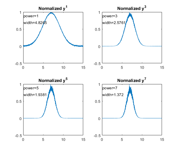 ng
more weight on the points near the peak, resulting in more nearly
Gaussian peak shapes (because most peak shapes are locally Gaussian
near the peak maximum) and smaller peak widths reducing the
width by the square root of the power). The technique is
demonstrated by the Matlab/Octave script PowerLawDemo.m,
shown in the figure on the left, which plots noisy Gaussians raised
to the power p=1 to 7, peak heights normalized to 1.0, showing that
as the power increases, peak width decreases and noise is reduced on
the baseline but increased on the peak maximum. Since the positions
of the peaks are not moved by this process, the peak resolution
(defined as the ratio of peak separation to peak width) is
increased. In the figure on the right, the blue line shows two
slightly overlapping peaks. The other lines are the result of
raising the data to the power of n = 2, 3, and 4, and
normalizing each to a height of 1.00. The peak widths, measured with
the halfwidth.m function, are 19.2, 12.4,
9.9, and 8.4 units for powers 1 through 4, respectively. For
Gaussian peaks, the area under the original peak can be calculated
from the area under the normalized power-sharpened curve (reference
63). . However, there is a complication: for a signal of two
overlapping Gaussians, the result of raising the signal to a power
is not the same as adding two power-narrowed Gaussians: simply, an+bn
is not the same as (a+b)n for n>1.
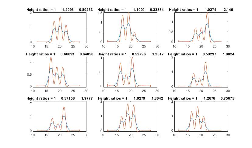
This
can
be demonstrated graphically by the script PowerPeaks.m
(graphic),
which curve-fits a two-Gaussian model to the power-raised sum of
two overlapping Gaussians; as the power n increases, the peaks
are narrowed anda the valley between them deepened, but the
resulting signal is no longer the sum of two Gaussians, unless the
resolution is sufficiently high.
ng
more weight on the points near the peak, resulting in more nearly
Gaussian peak shapes (because most peak shapes are locally Gaussian
near the peak maximum) and smaller peak widths reducing the
width by the square root of the power). The technique is
demonstrated by the Matlab/Octave script PowerLawDemo.m,
shown in the figure on the left, which plots noisy Gaussians raised
to the power p=1 to 7, peak heights normalized to 1.0, showing that
as the power increases, peak width decreases and noise is reduced on
the baseline but increased on the peak maximum. Since the positions
of the peaks are not moved by this process, the peak resolution
(defined as the ratio of peak separation to peak width) is
increased. In the figure on the right, the blue line shows two
slightly overlapping peaks. The other lines are the result of
raising the data to the power of n = 2, 3, and 4, and
normalizing each to a height of 1.00. The peak widths, measured with
the halfwidth.m function, are 19.2, 12.4,
9.9, and 8.4 units for powers 1 through 4, respectively. For
Gaussian peaks, the area under the original peak can be calculated
from the area under the normalized power-sharpened curve (reference
63). . However, there is a complication: for a signal of two
overlapping Gaussians, the result of raising the signal to a power
is not the same as adding two power-narrowed Gaussians: simply, an+bn
is not the same as (a+b)n for n>1.
This
can
be demonstrated graphically by the script PowerPeaks.m
(graphic),
which curve-fits a two-Gaussian model to the power-raised sum of
two overlapping Gaussians; as the power n increases, the peaks
are narrowed anda the valley between them deepened, but the
resulting signal is no longer the sum of two Gaussians, unless the
resolution is sufficiently high.
- it only works if the peaks of interest make a distinct maximum (it's not effective for side peaks that are so small that they only form shoulders; there must be a valley between the peaks);
- the baseline must be zero for best results;
- for noisy signals there is a decrease in signal-to-noise ratio because the smaller width means fewer data points are contributing to the measurement (smoothing can help).
- the method introduces severe non-linearity into the signal, changing the ratios between peak heights (as is evident in the figure above right) and complicating further processing, especially quantitative measurement calibration.|
However, there is an easy way to compensate for this
non-linearity in quantitative analysis application: after the raw
data have been raised to the power n and peaks
heights and/or areas have been measured, the resulting peak
measures can be simply raised to the power 1/n,
restoring the original linearity (but, notably, not the slope)
of the calibration curves
used in quantitative analytical measurements. (This works because
the peak area is proportional to the height times width, and peak
height of the power transformed peaks is proportional to
the nth power of the original height, but the width
of the peak is not a function of peak height at constant n,
thus the area of the transformed peaks remains proportional to nth
power of the original height). This technique is demonstrated
quantitatively for two variable overlapping peaks by the
Matlab/Octave script PowerLawCalibrationDemo.m
(graphic) which takes
the nth power of the overlapping-peak signal, measures
the areas of the power-narrowed peaks, and then takes the 1/n
power of the measured areas, constructing and using a calibration
curve to convert areas to concentration. Peak areas are measured
by perpendicular drop, using the half-way point to mark the
boundary between the peaks. The script simulates a mixture signal
with concentrations that you can specify in lines 15 and 16. You
can change the power and any of the parameters in lines 14-22. The
results show that the power method improves the accuracy of the
measurements as long as the 4-sigma resolution (the ratio of peak
separation to 4 times the sigma of the Gaussians) is above about
0.4. It is most accurate when the peaks are roughly equal in width
and when the ratio of the two concentrations are not very
different from the ratio in the standards from which the
calibration curve is constructed. Note that, even when the random
noise (in line 22) is zero, the results are not perfect due to
effect of peak overlap on area measurement, which varies depending
upon the ratio of two components in the mixture. (Requires gaussian.m, halfwidth.m,
val2ind.m, and plotit.m
downloaded from this web site).
The
self-contained function PowerMethodDemo.m demonstrates
the power method for measuring the area of small
shouldering peak that is partly overlapped by a much
stronger interfering peak (Graphic).
It shows the effect of random noise, smoothing, and any uncorrected
background under the peaks.
Combining sharpening methods. The
power method is independent of, and can be used in conjunction
with, the derivative methods discussed above.  However,
because the power method is non-linear, the order in
which the operations are performed is important. The first step
should be the first-derivative symmetrization if the signal is
exponentially broadened, the second step should be even-derivative
sharpening, and the power method should be used last. The reason
for this order is that the power method depends on, but can not
create, a valley between highly overlapped peaks. The
derivative methods may be able to create a valley between peaks if
the overlap is not too severe. Moreover, when used last, the power
method reduces the severity of baseline oscillations that are a
residue of the even-derivative sharpening (particularly noticeable
on a Lorentzian peak). The Matlab scripts SharpenedGaussianDemo2.m (Graphic) and SharpenedLorentzianDemo2.m
(Graphic on right) make
this point for Gaussian and Lorentzian peaks respectively,
comparing the result of even-derivative sharpening alone with
even-derivative sharpening followed by the power method (and
preforming the power method two ways, taking the square of the
sharpened peak or multiplying it by the original peak). For both
the Gaussian and Lorentzian original peak shapes, the final
sharpened results are fit to Gaussian models to show the changes
in peak parameters. The result is that the combination of methods
yields the narrowest final peak and the closest to Gaussian shape.
Of course, the linearity issues of the power method, if used,
remain.
However,
because the power method is non-linear, the order in
which the operations are performed is important. The first step
should be the first-derivative symmetrization if the signal is
exponentially broadened, the second step should be even-derivative
sharpening, and the power method should be used last. The reason
for this order is that the power method depends on, but can not
create, a valley between highly overlapped peaks. The
derivative methods may be able to create a valley between peaks if
the overlap is not too severe. Moreover, when used last, the power
method reduces the severity of baseline oscillations that are a
residue of the even-derivative sharpening (particularly noticeable
on a Lorentzian peak). The Matlab scripts SharpenedGaussianDemo2.m (Graphic) and SharpenedLorentzianDemo2.m
(Graphic on right) make
this point for Gaussian and Lorentzian peaks respectively,
comparing the result of even-derivative sharpening alone with
even-derivative sharpening followed by the power method (and
preforming the power method two ways, taking the square of the
sharpened peak or multiplying it by the original peak). For both
the Gaussian and Lorentzian original peak shapes, the final
sharpened results are fit to Gaussian models to show the changes
in peak parameters. The result is that the combination of methods
yields the narrowest final peak and the closest to Gaussian shape.
Of course, the linearity issues of the power method, if used,
remain.
Deconvolution. Another signal processing technique that can increase the resolution of overlapping peaks is deconvolution, which is treated in more detail here. It is applicable in the situation where the original shape of the peaks has been broadened and/or made asymmetrical by some broadening process or function. If the broadening process can be described mathematically or measured separately, then deconvolution from the observed broadened peaks is in principle capable of extracting the underlying peaks shape.
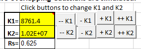 eadsheet will calculate K1
and K2. There is also a demonstration version with adjustable
simulated peaks which you can experiment with (PeakSharpeningDemo.xlsx and PeakSharpeningDemo.ods), as well
as a version that has clickable
ActiveX buttons (detail on left) for convenient interactive
adjustment of the K1 and K2 factors by 1% or by 10% for each
click.You can type in first estimates for K1 and K2 directly into
cells J4 and J5 and then use the buttons to fine-tune the values.
(Note: ActiveX buttons do not work in the iPad version of Excel). If
the signal is noisy, adjust the smoothing using the 17 coefficients
in row 5 columns K through AA, just as with the smoothing spreadsheets.
There is also a 20-segment version where the sharpening constants
can be specified for each of 20 signal segments (SegmentedPeakSharpeningDeriv.xlsx).
For applications where the peak widths gradually increase (or
decrease) with time, there is also a gradient peak
sharpening template (GradientPeakSharpeningDeriv.xlsx)
and an example with data (GradientPeakSharpeningDerivExample.xlsx);
you need only set the starting and ending peak widths and the
spreadsheet will apply the required sharpening factors K1 and K2.
eadsheet will calculate K1
and K2. There is also a demonstration version with adjustable
simulated peaks which you can experiment with (PeakSharpeningDemo.xlsx and PeakSharpeningDemo.ods), as well
as a version that has clickable
ActiveX buttons (detail on left) for convenient interactive
adjustment of the K1 and K2 factors by 1% or by 10% for each
click.You can type in first estimates for K1 and K2 directly into
cells J4 and J5 and then use the buttons to fine-tune the values.
(Note: ActiveX buttons do not work in the iPad version of Excel). If
the signal is noisy, adjust the smoothing using the 17 coefficients
in row 5 columns K through AA, just as with the smoothing spreadsheets.
There is also a 20-segment version where the sharpening constants
can be specified for each of 20 signal segments (SegmentedPeakSharpeningDeriv.xlsx).
For applications where the peak widths gradually increase (or
decrease) with time, there is also a gradient peak
sharpening template (GradientPeakSharpeningDeriv.xlsx)
and an example with data (GradientPeakSharpeningDerivExample.xlsx);
you need only set the starting and ending peak widths and the
spreadsheet will apply the required sharpening factors K1 and K2.

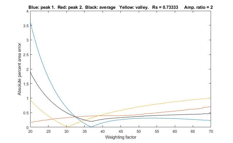 the errors of
measuring peak areas of two
overlapping Gaussians by the perpendicular
drop method using the autopeaks.m
function. It does this by applying different degrees of
sharpening and plotting the area errors (percent difference
between the true and measured errors) vs the sharpening
factor, as shown on the right. It also shows the height of the
valley between the peaks (yellow line). This demonstrates that
(1) the optimum sharpening factor depends upon the width and
separation of the two peaks and on their height ratio, (2)
that the degree of sharpening is not overly critical, often
exhibiting a broad optimum region, (3) that the optimum for
the two peaks is not necessarily exactly the same, and (4)
that the optimum for area measurement usually does not occur
at the point where the valley is zero. (To run this script you
must have gaussian.m, derivxy.m, autopeaks.m,
val2ind.m, and halfwidth.m
in the path. Download these from https://terpconnect.umd.edu/~toh/spectrum/).
the errors of
measuring peak areas of two
overlapping Gaussians by the perpendicular
drop method using the autopeaks.m
function. It does this by applying different degrees of
sharpening and plotting the area errors (percent difference
between the true and measured errors) vs the sharpening
factor, as shown on the right. It also shows the height of the
valley between the peaks (yellow line). This demonstrates that
(1) the optimum sharpening factor depends upon the width and
separation of the two peaks and on their height ratio, (2)
that the degree of sharpening is not overly critical, often
exhibiting a broad optimum region, (3) that the optimum for
the two peaks is not necessarily exactly the same, and (4)
that the optimum for area measurement usually does not occur
at the point where the valley is zero. (To run this script you
must have gaussian.m, derivxy.m, autopeaks.m,
val2ind.m, and halfwidth.m
in the path. Download these from https://terpconnect.umd.edu/~toh/spectrum/).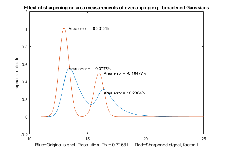 SymmetizedOverlapDemo.m
demonstrates the optimization of the first derivative
symmetrization for the measurement
of the areas of two overlapping exponentially broadened
Gaussians, shown on the left. It plots and compares the original
(blue) and sharpened peaks (red), then tries first-derivative
weighting factors from +10% to -10% of the correct tau value in
line 14) plots absolute peak area errors vs factor values. You
can change the resolution by changing either the peak positions
in lines 17 and 18 or the peak width in line 13. Change
height in line 16. Must have derivxy.m, autopeaks.m, and
halfwidth.m in the path.
SymmetizedOverlapDemo.m
demonstrates the optimization of the first derivative
symmetrization for the measurement
of the areas of two overlapping exponentially broadened
Gaussians, shown on the left. It plots and compares the original
(blue) and sharpened peaks (red), then tries first-derivative
weighting factors from +10% to -10% of the correct tau value in
line 14) plots absolute peak area errors vs factor values. You
can change the resolution by changing either the peak positions
in lines 17 and 18 or the peak width in line 13. Change
height in line 16. Must have derivxy.m, autopeaks.m, and
halfwidth.m in the path. you
can use the segmented version SegmentedSharpen.m, for which the input
arguments factor1, factor2, and SmoothWidth are vectors.
The script DemoSegmentedSharpen.m,
shown on the right, uses this function to sharpen four
Gaussian peaks with gradually increasing peak widths from left
to right with increasing degrees of sharpening, showing that
the peak width is reduced
by 20% to 22% compared to the original. DemoSegmentedSharpen2.m
shows four peaks of the same width sharpened to
increasing degrees. For asymmetrical peaks
whose exponential broadening varies across the signal, you can
use the symmetrize.m function described above in the same way:
specify "factor" and "smoothwidth" as vectors, just
like the segmented sharpening. And if peak widths and/or
exponential factors increase or decrease regularly across the
signal, you can simplify the calculation of these vectors by
giving only the number of segments ("NumSegments"), the first
value, "startv", and the last value, "endv", like so:
you
can use the segmented version SegmentedSharpen.m, for which the input
arguments factor1, factor2, and SmoothWidth are vectors.
The script DemoSegmentedSharpen.m,
shown on the right, uses this function to sharpen four
Gaussian peaks with gradually increasing peak widths from left
to right with increasing degrees of sharpening, showing that
the peak width is reduced
by 20% to 22% compared to the original. DemoSegmentedSharpen2.m
shows four peaks of the same width sharpened to
increasing degrees. For asymmetrical peaks
whose exponential broadening varies across the signal, you can
use the symmetrize.m function described above in the same way:
specify "factor" and "smoothwidth" as vectors, just
like the segmented sharpening. And if peak widths and/or
exponential factors increase or decrease regularly across the
signal, you can simplify the calculation of these vectors by
giving only the number of segments ("NumSegments"), the first
value, "startv", and the last value, "endv", like so: in
Matlab/Octave is performed by the function DEMSymm.m. It is demonstrated by the script DemoDEMSymm.m and its two variations (1, 2), which creates two overlapping double exponential
peaks from Gaussian originals, then calls the function
DEMSymm.m to perform the symmetrization, using a three-level plus-and-minus
bracketing technique to help you to determine the best values
of the two weighting factors by trial and error. In the
example on the left, there are three red and three green
bracketing lines produced by taus that are different
by 10%; in this case the middle of the three bracketing lines
is the optimum value.
in
Matlab/Octave is performed by the function DEMSymm.m. It is demonstrated by the script DemoDEMSymm.m and its two variations (1, 2), which creates two overlapping double exponential
peaks from Gaussian originals, then calls the function
DEMSymm.m to perform the symmetrization, using a three-level plus-and-minus
bracketing technique to help you to determine the best values
of the two weighting factors by trial and error. In the
example on the left, there are three red and three green
bracketing lines produced by taus that are different
by 10%; in this case the middle of the three bracketing lines
is the optimum value. 

Before Peak Sharpening in
iSignal After peak sharpening in
iSignal
 If you have a signal that is
exponentially broadened, you can remove that broadening (and
increase the symmetry of the peaks) by the weighted first-derivative
addition technique described here. Press Shift-Y and enter
an estimated weighting factor (e.g., start with the width of the
peak) then press "1" and "2" keys to change weighting
factor by 10% and "Shift-1" and "Shift-2" keys to
change by 1%. Increase the factor until the baseline after the peak
goes negative, then increase it slightly so that it is a low as
possible but not negative. Run the script iSignalSymmTest.m (graphic on left)
for a example signal with two overlapping exponentially broadened
Gaussians.
If you have a signal that is
exponentially broadened, you can remove that broadening (and
increase the symmetry of the peaks) by the weighted first-derivative
addition technique described here. Press Shift-Y and enter
an estimated weighting factor (e.g., start with the width of the
peak) then press "1" and "2" keys to change weighting
factor by 10% and "Shift-1" and "Shift-2" keys to
change by 1%. Increase the factor until the baseline after the peak
goes negative, then increase it slightly so that it is a low as
possible but not negative. Run the script iSignalSymmTest.m (graphic on left)
for a example signal with two overlapping exponentially broadened
Gaussians.Real-time peak sharpening in
Matlab is discussed in Appendix
Y.