The symbolic integration of functions and the calculation of
definite integrals are topics that are introduced in elementary
Calculus courses. The numerical integration of digitized signals
finds application in analytical signal processing mainly as a method
for measuring the areas under the curves of peak-type signals.
Peak area measurements are very
important in chromatography,
a class of chemical measurement techniques in which a mixture of
components is made to flow through a chemically-prepared tube or
layer that allows some of the components in the mixture to travel
faster than others, followed by a device called a detector
that measures and records the components after separation. Ideally,
the components are sufficiently separated so that each one forms a
distinct peak in the
detector signal as a function of time. The magnitude of the peaks
are calibrated
to the concentration of that component by measuring the peaks
obtained from "standard solutions" of known concentration. In
chromatography it is common to measure the area under the
detector peaks rather than the height of the peaks, because
peak area is less sensitive to the influence of peak broadening
(dispersion) mechanisms that cause the molecules of a specific
substance to be be diluted and spread out rather than being
concentrated on one "plug" of material as it travels down the
column. These dispersion effects, which arise from many sources,
cause chromatographic peaks to become shorter, broader, and in some
cases more unsymmetrical, but they have little effect on the
total area under the peak, as long as the total number of
molecules remains the same. If the detector response is linear with
respect to the concentration of the material, the peak area remains
proportional to the total quantity of substance passing into the
detector, even though the peak height is smaller. A
graphical example is shown on the left (Matlab/Octave
code), which plots detector signal vs time, where the blue curve represents the original
signal and the red curve shows
the effect of broadening by dispersion effects. The peak height is
lower and the width is greater, but the area under the
curve is almost exactly the same. If the extent of broadening
changes between the time that the standards are run and the
time that the unknown samples are run, then peak area
measurements will be more accurate and reliable than peak
height measurements. (Peak height will be proportional to the
quantity of material only if the peak width and shape are constant).
Another example with greater broadening: (script and graphic).
Peak area measurements are occasionally used also in spectroscopy,
for example in flow
injection analysis and in graphite furnace atomic absorption (reference
87). In that application,
calibration curves based on
area measurements are more linear than peak height
measurements because most of the area of a peak is measured when the
transient absorbance is less than maximum and where Beer's
Law is more strictly obeyed.
On the other hand, peak height measurements are simpler to make and
are less prone to interference by neighboring, overlapping peaks.
And a further disadvantage of peak area measurement is that the peak
start and stop points must be determined, which may be difficult
especially if the multiple peaks overlap. In principle, curve
fitting can measure the areas of peaks even then they overlap, but
that requires that the shapes of the peaks be known at least
approximately (however, see PeakShapeAnalyticalCurve.m
described in the Appendix).
Before computers, there were several methods
used to compute peak areas that sound strange by today's standards:
(a) plot the signal on a paper chart, cut out the
peak with scissors, then weigh the cut out piece on a
micro-balance compared to a square section of known area;
(b) count the grid squares under a curve recorded on
gridded graph paper,
(c) use a mechanical ball-and-disk
integrator,
(d) use geometry to compute the area under a triangle constructed with its sides
tangent to the sides of the peak, or
(e) compute the cumulative sum of the signal magnitude and
measure the heights of the resulting steps (see figure below).
But now that computing power is built into or connected to every
measuring instrument, more accurate and convenient digital methods
can be employed. However it is measured, the units of peak
area are the product of the x and y units. Thus, in a
chromatogram where the x is time in minutes and y is volts, the area
is in volts-minute. In absorption spectrum where the x isnm
(nanometers) and y is absorbance, the area has the units of
absorbance-nm. Because of this, the numerical magnitude of peak area
will always be different from that of the peak height. If you are
performing a quantitative analysis of unknown samples by means of a
calibration
curve, you must use the same method of measurement for both
the standards and the samples, even if the measurements are
inaccurate, as long as the error is the same for all standards and
samples (which is why an approximate method like triangle
construction works better than expected for quantitative analysis).
The best method for calculating the area under a peak depends
whether the peak is isolated or overlapped with other peaks or
superimposed on a non-zero baseline or not. For an isolated peak,
Yuri Kalambet (reference 71) has shown that the trapezoidal
rule area is efficient estimate of full peak area with
extraordinary low error, whereas Simpson's
rule is less efficient in full area integration. For a
Gaussian peak, the trapezoidal rule requires 0.62 points per
standard deviation (or 2.5 points
within the 4*sigma basewidth) to achieve an integration error
of only 0.1%. This is demonstrated by a digital simulation of the effect of
sampling rate (data density) on the accuracy of peak area
measurements for single isolated sparsely sampled Gaussian peaks
(below left).
Computing the cumulative sum will convert a series of peaks into a
series of steps, the height of each of which is proportional to the
area under that peak (above, right). But this works well only if the
peaks are well separated from each other and if the baseline is
zero. This is a commonly used method in proton NMR spectroscopy,
where the area under each peak or multiplet is proportional to the
number of equivalent hydrogen atoms responsible for that peak.
The
classical way to handle the overlapping peak problem is to draw
two vertical lines from the left and right bounds of the peak down
to the x-axis and then to measure the total area bounded by the
signal curve, the x-axis (y=0 line), and the two vertical lines,
shown the the shaded area in the figure on the left, below. This
is often called the perpendicular drop method; it's an
easy task for a computer, although tedious to do by hand. The left
and right bounds of the peak are usually taken as the valleys
(minima) between the peaks or as the point half-way between the
peak center and the centers of the peaks to the left and right.
The basic assumption is that the area missed by cutting off the
feet of one peak is made up for by including the feet of the
adjacent peak. This is accurate only of the peaks are symmetrical,
not too overlapped, and equal in height and in width. In addition,
the baseline must be zero; any extraneous background signal must
be subtracted before measurement. Using this method it is possible
to estimate the area of the second peak in the example below to an
accuracy of about 0.3%, but the last two peaks give errors greater
than 4%. As a rough rule, the valley between the peaks must be
quite low, perhaps a quarter or a fifth of the adjacent peak
height, for this method to be acceptable. Even so, this method is
widely used because there is no simple alternative. If
there is no valley between the peaks you need to measure, it's
possible to apply peak
sharpening techniques to narrow the peaks and deepen the
valley before the perpendicular drop measurement; see PeakSharpeningAreaMeasurementDemo.xlsm
(screen image).
Moreover, asymmetrical peaks that are the result of exponential
broadening can be narrowed and symmetricalized
by the weighted addition of its first derivative, making the
perpendicular drop area measurements much more
accurate. In both cases, it may be necessary to set the
strength of sharpening higher than previously recommended, if it
that is the only way to form a valley between peaks whose areas
you want to measure.
Peak
area measurement for overlapping peaks, using
the perpendicular drop method (left, shaded area) and
tangent skim method (right, shaded area).
In the case where a single peak is superimposed on a straight or
broadly curved baseline, you might use the tangent skim method,
which measures the area between the curve and a linear baseline
drawn across the bottom of the peak (e.g. the shaded area
in the figure on the right, above). In general, the hardest part
of the problem and the greatest source of uncertainty is
determining the shape of the baseline under the peaks and
determining when each peaks begins and ends. Once those are
determined, you subtract the baseline from each point between the
start and end points, add them up, and multiply by the x-axis
interval. Incidentally, smoothing a noisy signal does not change
the areas under the peaks, but it may make the peak start and stop
points easier to determine. The downside of smoothing is that
increases peak width and the overlap between adjacent peaks.
Numerical methods of peak sharpening, for example derivative sharpening and
Fourier deconvolution, can help
with the problem of peak overlap, and both of these techniques
have the useful property that they do not change the total area
under the peaks.
If the shape of peaks is known, the most general way to
measure the areas of overlapping peaks is to use some type of
least-squares curve fitting, as is discussed in the three
following sections (A, B, C).
If the peak positions, widths, and amplitudes are unknown,
and only the fundamental peak shapes are known, then the iterative least-squares method can
be employed. In many cases, even the background can be accounted
for by curve fitting.
For
gas chromatography and mass spectrometry specifically, Philip
Wenig's OpenChrom is an open source
data system that can import binary and textual chromatographic
data files directly. It includes methods to detect baselines and
to measure peak areas in a chromatogram. Extensive documentation
is available. It is available for Windows, Linux, Solaris and
Mac OS X. A screen shot is shown on the left (click to
enlarge). The program and its documentation is regularly updated
by the author.
Another freely-available open-source program for mass
spectroscopy is "Skyline"
from MacCoss Lab Software,
which is specifically aimed at reaction monitoring. Tutorials and
videos are available.
Peak area measurement
using spreadsheets. EffectOfDx.xlsx (screen image) demonstrates that the
simple equation sum(y)*dx accurately measures the peak area of an
isolated Gaussian peak if there are at least 4 or 5 points visibly
above the baseline (or 2.5 points
within the 4*sigma basewidth) and as long as you include the
points out to plus and minus at least 2 or 3 standard deviations of
the Gaussian. It also shows that an exponentially broadened Gaussian
needs to include more points on the tailing (right-hand, in this
case) side to achieve the best accuracy. EffectOfNoiseAndBaseline.xlsx (screen image) demonstrates
the effect of random noise and non-zero baseline, showing that the
area is more sensitive to non-zero baseline that the same amount of
random noise.
Using sharpening for overlapping peak area measurements.
There is a set of downloadable spreadsheets for perpendicular drop
area measurements of overlapping peaks using 2nd and 4th derivative
sharpening. Sharpening the peaks reduces the degree of overlap
and can greatly reduce the peak area measurement error errors made
by the perpendicular drop method. There is an empty template for you
to paste your data into (PeakSharpeningAreaMeasurementTemplate.xlsm),
an example version with sample data and settings already entered (PeakSharpeningAreaMeasurementExample.xlsm),
and a "demo" that creates and measures simulated data with known
areas (PeakSharpeningAreaMeasurementDemo.xlsm)
so you can see how sharpening effects area measurement accuracy.
There are very brief instructions in row 2 of each of these. Also,
there are mouse-over pop-up notes on many of the cells (indicated by
a red marker in the upper right corner of the cell). All three have
clickable ActiveX buttons for convenient interactive adjustment of
the K2 and K4 factors by 1% or by 10% for each click. Of course the
problem is knowing what values of the 2nd and 4th derivative
weighting factors (K1 and K2) to use. Those values depend on the
peak separation, peak width, and the relative peak height of the two
peaks, and they must be selected experimentally based on your
preferred trade-off between extent of sharpening and extent of
baseline upset. A good place to start for Gaussian peaks is
(sigma^2)/30 for the 2nd derivative factor and (sigma^4)/200 for the
4th derivative factor, where sigma is the standard deviation of the
Gaussian, then adjust to give the narrowest peaks without
significant negative dips. Don't assume that increasing the K's
until baseline resolution is achieved will always give the best area
accuracy. The optimum values depend on the ratio of peak heights: at
1:1, with equal widths and shapes, the perpendicular drop method
works perfectly with no sharpening, but if there is inequality in
shapes, heights, or widths, increased K values give lower errors up
to a point, but overdoing the sharpening can sacrifice
accuracy.
The two screen images screen1 and screen2,
which use the same K
values, show that it is possible to find K values that give
excellent accuracy for peak 2 over a range of relative peak
heights, even when the smaller peak is quite small. Without sharpening,
accurate perpendicular drop area measurements are impossible
because there is no valley between the peaks.
The symmetrization of exponentially broadened peaks by the
weighted addition of the first derivative is performed by the
template PeakSymmetrizationTemplate.xlsm
(graphic); PeakSymmetrizationExample.xlsm
is an example application with sample data already typed in. The
procedure here is first to adjust k1 to get the most symmetrical
peak shapes (judged by equal but opposite slopes on the leading and
trailing edges), then enter the start time, valley time, and end
time from the graph for the pair of peaks you want to measure into
cells B4, B5, and B6, and finally (optionally) adjust the second
derivative sharpening factor k2. The perpendicular drop areas of
those two peaks are reported in the table in columns F and G. These
spreadsheets have Active-X clickable buttons to adjust the first
derivative weighting factor (k1) in cell J4 and the second
derivative sharpening factor k2 (cell J5). There is also a demo
version that allows you to determine the accuracy of perpendicular
drop peak areas under different conditions by internally generating
overlapping peaks of known peak areas, with specified asymmetry
(B6), relative peak height (B3), width (B4), and noise (B5): PeakSymmetrizationDemo.xlsm
(graphic).
For peaks that have a more complex broadening behavior, the template
PeakDoubleSymmetrizationExample.xlsm
allows symmetrization of double exponential broadening (graphic). Peak area measurement using
Matlab and Octave.
Matlab and Octave have built-in
commands for the sum of elements ("sum", and the cumulative sum
"cumsum") and the trapezoidal numerical integration ("trapz").
For example, these three Matlab commands
>> x=-5:.1:5; >> y=exp(-(x).^2); >> trapz(x,y)
These lines accurately compute the area
under the curve of x,y (in this case an isolated Gaussian,
whose area is theoretically known to be the square
root of pi, sqrt(pi), which is 1.7725. If the interval between x
values, dx, is constant, then the area is
simply yi=sum(y).*dx. Alternatively,
the signal can be integrated using yi=cumsum(y).*dx, then the
area of the peak will be equal to the height of the
resulting step, max(yi)-min(yi)=1.7725.
The area of a peak is proportional
to the product of its height and its width, but the
proportionality constant depends on the peak shape. A pure
Gaussian peak with a peak height h
and full-width
at half-maximumw has
a
total area of 1.064467*h*w.
A Gaussian-Lorentzian blend with p percent Gaussian
character has an area of ((100- p)/100)*((pi/2).*w*h) + (p /100)*(1.064467*w*h). A pure Lorentzian
peak has a total area of (pi/2)*h*w. The
graphic LorentzianVsGaussian.png
comparesGaussian and Lorentzian
peaks of the same height and width. The Lorentzian has
more area in the outer wings, so if you measure the area of an
unknown peak using trapz, you have to measure over a very wide
range on both sides of the peak. To get an area within 1%, you
need to expand that to 64 times the FWHM! (See LorentzianAreaProblem.m,
graphic). Many real signals in
practice have too many peaks that are too close together to
allow the theoretical areas to be measured directly by
integration. If you really need an accurate area and the
available measurement span is insufficient, it may be more
accurate to calculate the area analytically using the above
analytical expressions.
For a peak of any smooth shape on a zero baseline, the peak
width (FWHM) can be measured by my halfwidth.m
function.
But the peaks in real signals have some complications:
(a) their shapes might not be known;
(b) they may be superimposed on a baseline; and
(c) they may be overlapped with other peaks.
These must be taken into account to measure accurate areasin
experimental signals.Various Matlab/Octave
functions have been developed to deal with these complications.
Overlapping peaks. The following Matlab/Octave code uses
the perpendicular drop (PD) method to measure the areas of two
overlapping symmetrical peaks in the data vectors x,y by the
perpendicular drop method. Variables "m1" and "m2" are the
estimated positions of the two peaks. The "val2ind"
function returns the index number of the value in a vector that
value matches the specified value.
The third
line finds the half-way point between the two peaks. The last
two lines use the trapz function to measure the areas before and
after the valley point. index1=val2ind(x,m1); index2=val2ind(x,m2); valleyindex=val2ind(x,(m1+m2)/2), PDMeasArea1=trapz(x(1:valleyindex),y(1:valleyindex)); PDMeasArea2=trapz(x(valleyindex:length(x)),y(valleyindex:length(x)); Alternatively,
you could replace "valleyindex" with valleyy=min(y(index1:index2));
valleyindex=val2ind(y,valleyy);
which uses the minimum
between the peaks rather than the half-way point. But the
half-way point method has the advantage that the SNR at a
signal maximum is usually better than at a minimum,
so it's likely that maxima are more precisely located that
minima. Moreover, the half-way
point method works even when the overlap is so great
that there is not a discernible minimum between the peaks. My
function PerpDropAreas.m
uses the half-way point method to measure the areas of any
number of overlapping peaks, given a list of their peak maxima
positions. These methods work best if the peak widths are not very
different.
Although the perpendicular drop method remains
popular, there are other geometrical methods that can work
better in many cases. The "equalization" method, illustrated in
the figure on the left, uses another method of locating the
perpendicular drop point. A line of three straight-line segments
is
constructedthat
touches the estimated maxima of the two peaks,
shown by the dotted red line called the
"cline" in the figure on the left. The quotient
of the original signal, in blue, divided by this line, results
in a temporarily normalized signal (the yellow line) that has
more nearly equal peak heights. The
effect of this treatment is to deepen the valley between
the peaks, so
that it remains distinct for lower values of
the second peak height. This
is used only for the purpose of determining its
minimum, shown as a vertical black line, and then is
discarded. Using that minimum as the
separation point between the peaks, the perpendicular
drop areas are then calculated on the
original observed signal (blue line).
Note that this new valley point is not quite the same as the
valley of the original signal, nor is it the half-way point
between the two peak positions. The process need not be done
by hand; it is easily automated, given only an initial
estimate for the two peak positions based on the observed
signal. The Matlab/Octave function EqualPerpDrop.m performs the
calculation; the script EqualPerpDropTest.m
demonstrates the use of the function applied to the
measurement of two simulated overlapping EMG (exponentially
modified Gaussian) peaks.
The
"reflection/subtraction" method, shown on the right, is simpler.
As before, the original signal is shown in blue. An estimate of the
isolated first (larger) peak is constructed by reflecting its
left half and using it to replace the right half, resulting in
the red dotted line in the figure, assuming that the first peak
is symmetrical. Then that peak is simply subtracted from the
entire signal to reveal the isolated second peak (dotted yellow
line). The two areas are then separately calculated by the
"trapz" function. This process is also easily automated, given
only the peak position of the first peak. It works perfectly
only if the first peak is the larger of the two peak and is
symmetrical and if
the peak separation is sufficient so that the left-hand tail
of the smaller peak does not significantly increase the
height of the first peak.
So, how do these new methods compare to the traditional
perpendicular drop method? Matlab/Octave code for all of these
methods is contained in the script "OverlapAreaComparison.m"
which compares the accuracy of several methods of peak area
measurement for two simulated partially overlapped Gaussian
peaks with variable height ratios and resolutions. (There is
also an interactive Live Script version
of this script.) For the case of Gaussian peak with a resolution
of 0.7 and a height ratio of 1 to 0.5, the relative percent
error of the peak areas are:
You can
change the parameters in lines 5 through 10 to test with other
peak separations and relative peak heights. The equalization
method is often, but not always, the most accurate method.
(Note: the
script requires the downloadable functions val2ind.m, halfwidth.m,
ExpBroaden.m, and plotit.m functions be in the path).
A more through investigation
of these methods demonstrates the effect of changing the
peak resolution, shown on the left (script,
graphic)
and of changing the the height of the smaller peak, shown on
the right (script, graphic).
These scripts include the effect of random noise in
the signal, because noise can influence the location of peak
maxima and the separation point between the peaks, whether
they are determined manually or by a computer algorithm (as
it is here);
the
random noise is set by the variable
"noise", which is the fractional
random white noise added to the
signal. Also,
these scripts include the effect ofasymmetry of the peak shapes, which
can cause errors in area measurement by all
these methods. After all, the very reason
for measuring peak area rather than peak
heights is to reduce
the effect of uncontrolled variations in
peak broadening.
The asymmetry is set by the variable "TimeConstant",
which is the time constant of the exponential
convolution applied to the signal that reduces the
height and stretches out the right-hand half. Both
of those are zero in the above figures for
simplicity and to show the best possible accuracy.
For example, with a resolution of 1.0, a tau of 2,
and noise set to 0.01 (1%),
the valley perpendicular drop and the equalization method
outperform the other methods (graphic). Things are much easier and
more forgiving in quantitative analysis, using a calibration curve,
because in
that case absolute area
accuracy is not really necessary. Rather, it is really the
reproducibility of the areas that is key. Systematic errors
in the area measurement simply change the slope of
the calibration curve, and as long as the conditions are the
same between calibration and analysis (always a requirement
in any case), the error will cancel out exactly. For
example, if you run the above scripts with very asymmetrical
peaks (TimeConstant=3), poor resolution (resolution
=0.68), and visible amounts of random noise=5%, the
systematic area measurement errors
are quite large (5%-15%), but nevertheless
good linear calibration curves are produced by both
the halfway point
perpendicular drop and the equalization method, over
the range of relative peak heights
of 0.1 to 0.99, with
correlation coefficients of 0.999. All
of these methods produce significant
errors if the peaks are highly
overlapped or asymmetrical. However,
asymmetry that is the
result of exponential broadeningcan
be
symmetrized before computing
the areas using the first
derivative addition method,
which sharpens the peaks and removes
the asymmetry without changing
the peak areas. Other methods
of peak sharpening, especially self-deconvolution,
can also be used when the peak to be
measured is too weak or too poorly
resolved to allow easy measurement.
Ultimately,
in the most difficult cases, you may
have to consider the use of iterative
curve fitting, though it is
admittedly more complex
mathematically and is subject to its
own limitations. Automatic multiple peak
detection
Measurepeaks.m is a
function that quickly and automatically detects peaks
in a signal,
using the derivative zero-crossing method described previously,
and measures their areas using the perpendicular drop and
tangent skim methods. It shares the first 6 input arguments with
findpeaksSG.
The syntax is M=measurepeaks(x,y, SlopeThreshold,
AmpThreshold, SmoothWidth, FitWidth, plots). It returns a
table containing the peak
number, peak
position, absolute peak
height, peak-valley difference,
perpendicular drop area, and the tangent skim area of
each peak it detects. If
the last input argument ('plots') is set to 1, it plots the signal
with numbered peaks (shown
on the left)
and also plots the individual peaks (in
blue) with the maximum (red circles), valley points (magenta),
and tangent lines (cyan) marked as shown
on the right. Type "help measurepeaks" and try the
seven examples there, or run HeightAndArea.m
to test the accuracy of peak
height and area measurement with signals that have
multiple peaks with noise, background, and some peak overlap.
Generally, the values for
absolute
peak height and perpendicular
drop area are best for peaks that have no background, even
if they are slightly overlapped, whereas the values for peak-valley
difference and for tangential
skim area are better for isolated peaks on a straight or
slightly curved background. Note: this function uses smoothing (specified by the
SmoothWidth input argument) only for peak detection;
it performs measurements on the raw unsmoothed y
data. If the raw data are noisy, it may be beneficial to
smooth the y data yourself before calling measurepeaks.m,
using any smooth function of your choice.
[M,A]=autopeaks.m
is basically a combination or autofindpeaks.m and
measurepeaks.m. It has similar syntax to measurepeaks.m,
except that the peak detection parameters (SlopeThreshold,
AmpThreshold, smoothwidth peakgroup, and smoothtype)
can be omitted and the function will calculate trial values
in the manner of autofindpeaks.m.
Using the simple syntax [M,A]=autopeaks(x,
y) works well in some cases, but if not
try [M,A]=autopeaks(x,
y, n), using different values of n
(roughly the number of peaks that
would fit into the signal record) until it
detects the peaks that you want to
measure. Like
measurepeaks, it returns a table
M containing the peak number, peak
position,
absolute peak
height, peak-valley difference,
perpendicular drop area, and tangent
skim area of each peak it detects, but is
also can optionally return a
vector A containing the peak detection
parameters that it calculates (for use
by other peak detection and fitting functions).
For the most precise
control over peak detection, you can
specify all the peak detection parameters
by typing M=autopeaks(x,y, SlopeThreshold,
AmpThreshold, smoothwidth, peakgroup).
[M,A]=autopeaksplot.m is the
same but it also plots the signal and the individual peaks
in the manner of measurepeaks.m (shown above).
The script testautopeaks.m
runs all the examples in the autopeaks help file, with a 1-second
pause between each one, printing out results in the command window
and additionally plotting and numbering the peaks (Figure window
1) and each individual peak (Figure window
2); it requires gaussian.m and
fastsmooth.m in the path.
Peak sharpening, introduced previously, can often help
in the measurement of the areas of overlapping peaks, by creating
(or deepening) the valleys between peaks that are needed by the
perpendicular drop method. SharpenedOverlapDemo.m is a
script that automatically determines the optimum degree of
even-derivative sharpening that minimizes the errors of
measuring peak areas of two
overlapping Gaussiansby the perpendicular drop
method using the autopeaks.m function.
It does this by applying different degrees of sharpening and
plotting the area errors (percent difference between the true and
measured errors) vs the sharpening factor, as shown on the right.
It also shows the height of the valley between the peaks (yellow
line). This demonstrates that (1) the optimum sharpening factor
depends upon the width and separation of the two peaks and on
their height ratio, (2) that the degree of sharpening is not
overly critical, often exhibiting a broad optimum region, (3) that
the optimum for the two peaks is not necessarily exactly the same,
and (4) that the optimum for area measurement usually does not
occur at the point where the valley is zero. (To run this script
you must have gaussian.m, derivxy.m, autopeaks.m,
val2ind.m, and halfwidth.m
in the path. Download these from https://terpconnect.umd.edu/~toh/spectrum/).
SharpenedOverlapCalibrationCurve.m
is a script that simulates the construction and use of calibration
curves of three overlapping Gaussian peaks (the blue lines in the
signal plots on the left) . Even-derivative sharpening (the red line
in the signal plots) is used to improve the resolution of the peaks
to allow perpendicular drop area measurement. A straight line is fit to the
calibration curve and the R2 is calculated, in order to demonstrate
(1) the linearity of the response, and (2) in independence of the
overlapping adjacent peaks. You can easily change:
1. The resolution, Rs, by changing the peak width
w in line 15. Default is w=2, Rs=0.55
2. The peak ratios, by changing the minimum and
maximum peaks in lines 21 and 22. Default is 0.2 and 1.0. (1:5 ratio
range)
3. The number of standards in line 24. Larger
numbers give a more reliable calibration curve.
4. The number of simulated samples, line 25.
Larger numbers give more reliable average errors.
SymmetrizedOverlapCalibrationCurve.m
is the same thing for symmetrization of overlapping exponentially
modified Gaussian peaks by first-derivative addition. The critical
variable is "factor" in line 27, which for best results should match
or slightly exceed "tau", the exponential time constant in line 19.
To compare to using the original signal, set "factor" to 0.1. You
must have gaussian.m, derivxy.m,
autopeaks.m,
val2ind.m, halfwidth.m,
fastsmooth.m, and plotit.m
in the path for either of these two scripts.
The Matlab/Octave automatic peak-finding function findpeaksG.m
computes peak area assuming that the peak peak shape is Gaussian (or
Lorentzian, for the variant findpeaksL.m).
The related function findpeaksT.m
uses the triangle construction method to compute the peak
parameters. Even for well-separated Gaussian peaks, the area
measurements by the triangle construction method is not very
accurate; the results are about 3% below the correct
values. (But this method does perform better than findpeaksG.m when
the peaks are noticeably asymmetric; see triangulationdemo for some examples). In contrast, measurepeaks.m makes no assumptions
about the shape of the peak.; it simply looks for the minima on
both sides of each peak to use as the dividing point between
peaks. iSignal(shown on the left) is
a downloadable interactive multipurpose signal processing Matlab
function that includes various signal processing functions
described in this tutorial, including measurement of peak area
using Simpson's Rule and the perpendicular drop method. Click to
view or right-click > Save
link as...here, or you can download theZIP filewith sample data
for testing. It is shown on the left applying
the perpendicular drop method to a series of four peaks of
equal area. (Look at the bottom panel to see how the
measurement intervals, marked by the vertical dotted magenta
lines, are positioned at the valley minimum on
either side of each of the four peaks).
Here's a bit of Matlab/Octave code that creates
four computer-synthesized Gaussian peaks,similar to this figure,
that all have the same height (1.000), width (1.665),
and area (1.772) but with different degrees of peak
overlap: x=[0:.01:18];
y=exp(-(x-4).^2) + exp(-(x-9).^2) + exp(-(x-12).^2) +
exp(-(x-13.7).^2);
isignal(x,y);
To use iSignal to
measure the areas of each of these peaks by the perpendicular drop
method, use the pan and zoom keys to position the two outer cursor
lines (dotted magenta lines) in the valley on either side of the
peak. The total of each peak area will be displayed below the upper
window.
The area results are reasonably accurate in this
example only because the perpendicular drop method roughly
compensates for partial overlap between peaks, but only if the
peaks are symmetrical, about equal in height, and have zero
background.
Peak area measurements by multiple
methods is a part of the Live Script Peak detection tool PeakDetection.mlx
described here
and illustrated on the left. This interactive tool allows optional
first-derivative
symmetrization of skewed peaks, as well as symmetrical
sharpening by Fourier
self-deconvolution, to enhance the resolution of overlapping
peaks and improve the accuracy of peak are measurement.
iSignal version 5.9 includes an additional command (J key)
that calls the autopeaksplot function,
which automatically detects the peaks in the signal and measures
their peak position, absolute peak height, peak-valley difference,
perpendicular drop area, and tangent skim area. It asks you to type
in the peak density (roughly the number of peaks that would fit into
the signal record); the greater this number, the more sensitive it
is to narrow peaks. It displays the measured peaks just as does the
measurepeaks function described above. (To return to iSignal, press
any cursor arrow key).
Area measurement by iterative curve
fitting. In general, the most flexible peak area measurements
for overlapping peaks, assuming that the basic shape of the peaks is known or
can be guessed, are made with iterative
least-squares peak fitting, for example using peakfit.m, shown on the
right (for Matlab and Octave).
This function can fit any number of overlapping peaks with model
shapes selected from a list of different types. It uses the "trapz"
function to calculate the area of each of the component mode peak.
For example, using the peakfit function on the same
data set as above, the results are much more accurate:
iPeak can
also be used to estimate peak areas. It uses the same Gaussian curve
fitting method as iSignal,
but it has the advantage that it can detect and measure all the
peaks in a signal in one operation. For example:
Peaks 1 and 2 are measured accurately by iPeak, but the peak
widths and areas for peaks 3 and 4 are not accurate because of the
peak overlap. Fortunately, iPeak has a built-in
"peakfit" function (activated by the N key) that uses these peak position and width
estimates as its first guesses, resulting in good accuracy for all
four peaks.
The Live Script Peak detection tool PeakDetection.mlx,
described here, also
includes optional iterative least-squares curve fitting. Correction
for background/baseline. The
presence of a baseline or background signal, on which the peaks are
superimposed, will greatly influence the measured peak area if not
corrected or compensated. iSignal,
iPeak, measurepeaks, and peakfitall have
several different baseline correction modes, for flat, linear, and
quadratic baselines, and iSignal
and iPeak have a
multipoint piece-wise linear baseline subtraction function allows
the manually estimated background to be subtracted from the entire
signal. See iSignal.html#background_subtraction,
ipeakdemo1 on PeakFindingandMeasurement.htm#demos,
and CurveFittingC.html#Background_correction
for examples of these background correction functions. If the
baseline is actually caused by the edges of a strong overlapping
adjacent peak, then it's possible to include that peak in the
curve-fitting operation, as see in Example 22 on InteractivePeakFitter.htm.
The script AreasOfIsolatedPeaks2.m
demonstrates the use of peakfit.m for a simulated experimental
signal consisting of several isolated peaks on a straight tilted
baseline. In this example, the positions of the peaks are assumed to
have been previously measured by a peak detector algorithm
and to be reproducible enough that a pre-determined set of
measurement segments can be used to fit each peak separately and
determine its position, height, width, and area.
Here's a Matlab/Octave experiment that compares several different
methods of baseline correction in peak area measurement. The
signal consists of two noiseless, slightly overlapping Gaussian
peaks with theoretical peak heights of 2.00 and 1.00 and areas of
191.63 and 95.81 units, respectively. The baseline is tilted and
linear, and slightly greater in magnitude than the peak heights
themselves, but the most serious problem is that the signal
never returns to the baseline long enough to make it easy to
distinguish the signal from the baseline.
iSignal, using perpendicular drop in baseline mode 1, seriously
underestimates both peak areas (168.6 and 81.78).
An automated tangent skim measurement by measurepeaks
is not accurate in this case because the peaks do not go all the way
down to the baseline at the edges of the signal and because of the
slight overlap:
>> measurepeaks(x,y,.0001,.8,2,5,1) Position
PeakMax Peak-valley Perp drop Tan skim 1 503.67
4.5091
1.895
672.29 171.44 2 707.44
4.5184
0.8857
761.65 76.685
An attempt to use curve fitting with peakfit.m in the flat
baseline correction mode 3 - peakfit([x;y],0,0,2,1,0,1,0,3),
above, left-most figure - does not really work because the
actual baseline is tilted, not flat. The linear baseline mode does a
little better (peakfit([x;y],0,0,2,1,0,1,0,1),
second figure from left) but it's not perfect in this case. A more
accurate approach is to fit the baseline as a third "peak" of a
different shape, with either a Lorentzian model - peakfit([x;y],0,0,3,[1
1 2]), third signal from the left - or with a "slope" model -
shape 26 in peakfit version 6, last figure on the right. The latter
method gives both the lowest fitting error (less than 0.01%) and the
most accurate peak areas (less than 1/2% error in peak area): >> [FitResults,FitError]=peakfit([x;y],0,0,3,[1
1 26]) FitResults =
1
500
2.0001
90.005 190.77
2
700
0.99999
89.998 95.373
3 5740.2
8.7115e-007
1 1200.1
FitError =0.0085798
Note that in this last case the number of peaks is 3 and the
shape argument is a vector [1 1 26] specifying two Gaussian
components plus the "linear slope" shape 26. If the baseline seems
to be non-linear, you might prefer to model it using a quadratic
(shape 46; see example 38 on InteractivePeakFitter.htm#Examples).
If the baseline seems to be different on either side of the
peak, try modeling the baseline with an S-shape (sigmoid), either an
up-sigmoid, shape 10(click for graphic),peakfit([x;y],0,0,2,[1 10],[0 0]), or a down-sigmoid, shape 23(click for graphic),peakfit([x;y],0,0,2,[1 23],[0 0]),
in these examples leaving the peak modeled as a Gaussian.Asymmetrical
peaks and peak broadening: perpendicular drop vs curve fitting.
AsymmetricalAreaTest.m
is a Matlab/Octave script that compares the accuracy of peak
area measurement
methods for a single
noisy asymmetrical peak
measured by different methods: (A) Gaussian estimation,(B)
triangulation, (C) perpendicular drop method, and
curve fitting by
(D) exponentially broadened
Gaussian, and (E) two overlapping Gaussians. AsymmetricalAreaTest2.m
is similar except that it compares the precision
(standard deviation) of the areas. For a single peak
with zero baseline, the
perpendicular drop and curve fitting
methods work equally well, both considerably better
than Gaussian estimation or triangulation. The
advantage of the curve fitting methods is that they
can deal more accurately with peaks that overlap or
that are superimposed on a baseline.
Here's a Matlab/Octave experiment that simulates a signal containing
five Gaussian peaks with the same initial peak height (1.0)
and width (3.0) but which are subsequently broadened by increasing
degrees of exponential broadening, similar to the broadening
of peaks commonly encountered in chromatography:
The theoretical area under these
Gaussians is all the same: 1.0645*Height*Width =
1*3*1.0645= 3.1938. A perfect area-measuring algorithm
would return this number for all five peaks.
As
the broadening is increased from left to right, the peak
height decreases (by about 35%) and peak width increases
(by about 32%). But because the area under the peak is
proportional to the product of the peak height and the
peak width, these two changes
approximately cancel each other out and the result is that
the peak area is nearly independent of peak broadening (see the
summary of results in 5ExponentialBroadenedGaussianFit.xlsx). The Matlab/Octave peak-finding function findpeaksG.m,
finds all five peaks and measures their areas assuming a Gaussian
shape; this works well for the unbroadened peak 1 (script), but it underestimates the
areas as the broadening increases in peaks 2-5:
The triangle construction method (using findpeaksT.m)
underestimates even the area of the unbroadened peak 1 and is less
accurate for the broadened peaks (script; graphic):
Using iSignal
and the manual peak-by-peak perpendicular drop method yields areas
of 3.193, 3.194, 3.187, 3.178, and 3.231, a mean of 3.1966
(pretty close to the theoretical value of 3.1938) and standard
deviation of only 0.02 (0.63%). Alternatively, integrating the signal, cumsum(y).*dx), where dx is the difference between adjacent x-axis values (0.1 in this
case), and then measuring the heights
of the resulting steps, gives similar results: 3.19, 3.19,
3.18, 3.17, 3.23. By either method, the peak heights are very
different but the areas are closer together, yet not exactly
equal.
But we can obtain a more accurate automated measurement of all
five peaks by iterative curve fitting, using peakfit.m
with multiple shapes, one Gaussian and four exponentially modified
Gaussians (shape 5) with different exponential factors (extra
vector):
>>
[FitResults,FittingError]=peakfit([x;y],30,54,5,[1 5 5 5
5],[0 -5 -10 -15 -20],10, 0, 0) FitResults = Peak# Position
Height
Width Area 1
9.9933
0.98051
3.1181 3.2541 2
20.002
1.0316
2.8348 3.1128 3
29.985
0.95265
3.233 3.2784 4
40.022
0.9495
3.2186 3.2531 5
49.979
0.83202
3.8244 3.2974 FittingError = 2.184%
The results in this case are disappointing; the fitting error is
not much better than the simple Gaussian fit.
Better results can be had using preliminary position and width
results obtained from the findpeaks
function or by curve fitting with a simple Gaussian fit and
using those results as the "start" vector:
Even more accurate results for area are obtained using peakfit
with one Gaussian and four equal-width exponentially
modified Gaussians (shape 8):
>> [FitResults,FittingError]=peakfit([x;y],30,54,5,
[1 8 8 8 8], [0 -5 -10 -15 -20],10, [10 3.5 20 3.5 31 3.5 41
3.5 51 3.5],0) FitResults = Peak# Position
Height
Width Area 1 10
1.0001
2.9995 3.1929 2 20
0.99998
3.0005 3.1939 3 30
0.99987
3.0008 3.1939 4 40
0.99987
2.9997 3.1926 5 50
1.0006
2.9978 3.1207 FittingError = 0.008%
The latter approach works
because, although the broadened peaks clearly have
different widths (as shown in the simple Gaussian fit), the
underlying pre-broadening peaks have all the same width.
In general, if you expect that the peaks should have equal widths,
or fixed widths, then it's better to use a constrained
model that fits that knowledge; you'll get better
estimates of the measured unknown properties, even though the
fitting error will be higher than for an unconstrained model.
The disadvantages of the exponentially-broadened model are
that (a) it may not be a perfect match to the actual physical
broadening process; (b) it's slower that a simple Gaussian
fit, and (c) it sometimes need help, in the form of a start vector
or equal-widths constraints, as seen above, in order to get the best
results.
Alternatively, if the objective is only
to measure the peak areas, and not the peak positions and
widths, then it's not even necessary to model the physical
peak-broadening of each peak. You can simply aim for a good fit
using two (or more) closely-spaced simple Gaussians for each peak
and simply add up the areas of the best-fit model. For
example, the 5th peak in the above example (the most
asymmetrical), can be fit very well with two overlapping Gaussians,
resulting in a total area of 1.9983+1.1948 = 3.1931, very close
to the theoretical area of 3.1938. Even more overlapping Gaussians can be
used if the peak shape is more complex.
This is called the "sum
rule" in integral
calculus: the integral of a sum of two functions is
equal to the sum of their integrals. As a
demonstration, the script SumOfAreas.m is shows that
even drastically
non-Gaussian peaks can be fit with multiple Gaussian components, and that the
total area of the components approaches the area under the non-Gaussian
peak as the number of components increases (graphic).
When using this technique, it's best to set the number of trials (NumTrials, the 7th input argument of the
peakfit.m function) to
10 or more; additionally, if the peak of interest is on a
baseline, you must add up the areas of only those peak that
contribute to fitting the peak itself and not those
that are fitting the baseline.
By stimulating a case
where the peaks are closer together, we can create a
tougher and more realistic challenge. y=modelpeaks2(x,[1 5 5 5 5],[1 1 1 1 1],[20 25 30 35
40],[3 3 3 3 3],[0 -5 -10 -15 -20]); In this case, the triangle
construction method gives areas of [3.1294 3.2020 3.3958
4.1563 4.4039], seriously overestimating the areas of the last two
peaks, and measurepeaks.m using the perpendicular drop method gives
areas of [3.233 3.2108 3.0884 3.0647 3.3602], compared to the theoretical value of 3.1938, better
but not perfect. The integration/step height method is almost useless because the steps are no longer
clearly distinct. The peakfit function does better, again
using the approximate result of findpeaksG.m to supply a
customized 'start' value.
Next, we simulate an even tougher challenge
with different peak heights (1, 2, 3, 4 and 5,
respectively) and a bit of added random noise. The theoretical
areas (Height*Width*1.0645)
are 3.1938, 6.3876, 9.5814, 12.775, and 15.969.
y=modelpeaks2(x,[1 5 5 5 5],[1 2 3 4 5], [20 25 30 35
40], [3 3 3 3 3], [0 -5 -10 -15 -20])+.01*randn(size(x));
>> [FitResults,FittingError]=peakfit([x;y],30,54,5, [1 8 8 8
8], [0 -5 -10 -15 -20] ,20, [20 3.5 25 3.5 31 3.5 36 3.5 41
3.5],0)
FitResults =
1
19.999
1.0015
2.9978 3.1958
2
25.001
1.9942
3.0165 6.4034
3 30
3.0056
2.9851 9.5507
4
34.997
3.9918
3.0076 12.78
5
40.001
4.9965
3.0021 15.966
FittingError =
0.2755
The measured areas in this case
(last column) are very close to to the theoretical values, whereas all the other methods give substantially poorer accuracy. The
more overlap between peaks, and the more unequal are the peak
heights, the poorer the accuracy of the perpendicular drop and
triangle construction methods. If the peaks are so overlapped that
separate maxima are not visible, both methods fail completely,
whereas curve fitting can often retrieve a reasonable result, but only
if approximate first-guess values can be supplied. The more
you give, the more you get.
First-derivative symmetrization.
Although curve fitting is generally the most powerful method for
dealing with the combined effects of overlapping asymmetrical peaks
superimposed on an irrelevant background, the simpler technique of first derivative
sharpening can be useful as a method to reduce or eliminate
the effects of exponential broadening, resulting in a simpler shape
that is easier to fit. This is a simple techniques that calculates
the weighted sum of the original signal and its first derivative.
You just vary different first derivative weighting factor and choose
the one that makes the baseline after the peaks as low as possible
without going negative. As is the case with curve fitting, it's most
convenient is there is also isolated peak with the same exponential
broadening, because that peak can be used to determine more easily
the best value of the first derivative weighting factor.
SymmetizedOverlapDemo.m,
illustrated on the left, demonstrates the optimization of the first
derivative symmetrization for the measurement of the areas of two
overlapping exponentially broadened Gaussians. It plots and compares
the original (blue) and sharpened peaks (red), then tries
first-derivative weighting factors from +10% to -10% of the correct
tau value in line 14) plots absolute peak area errors vs factor
values. You can change the resolution by changing either the peak
positions in lines 17 and 18 or the peak width in line 13.
Change height in line 16. Must have derivxy.m, autopeaks.m,
and halfwidth.m in the path. This method also easily deals with double exponential
broadening, which is not easily handled by curve fitting. This page is part of "A Pragmatic
Introduction to Signal Processing", created and
maintained by Prof. Tom
O'Haver , Department of Chemistry and Biochemistry, The
University of Maryland at College Park. Comments, suggestions and
questions should be directed to Prof. O'Haver at toh@umd.edu.
Updated May, 2023.
Unique visits since May 17, 2008:
 the
detector signal as a function of time. The magnitude of the peaks
are calibrated
to the concentration of that component by measuring the peaks
obtained from "standard solutions" of known concentration. In
chromatography it is common to measure the area under the
detector peaks rather than the height of the peaks, because
peak area is less sensitive to the influence of peak broadening
(dispersion) mechanisms that cause the molecules of a specific
substance to be be diluted and spread out rather than being
concentrated on one "plug" of material as it travels down the
column. These dispersion effects, which arise from many sources,
cause chromatographic peaks to become shorter, broader, and in some
cases more unsymmetrical, but they have little effect on the
total area under the peak, as long as the total number of
molecules remains the same. If the detector response is linear with
respect to the concentration of the material, the peak area remains
proportional to the total quantity of substance passing into the
detector, even though the peak height is smaller. A
graphical example is shown on the left (Matlab/Octave
code), which plots detector signal vs time, where the blue curve represents the original
signal and the red curve shows
the effect of broadening by dispersion effects. The peak height is
lower and the width is greater, but the area under the
curve is almost exactly the same. If the extent of broadening
changes between the time that the standards are run and the
time that the unknown samples are run, then peak area
measurements will be more accurate and reliable than peak
height measurements. (Peak height will be proportional to the
quantity of material only if the peak width and shape are constant).
Another example with greater broadening: (script and graphic).
the
detector signal as a function of time. The magnitude of the peaks
are calibrated
to the concentration of that component by measuring the peaks
obtained from "standard solutions" of known concentration. In
chromatography it is common to measure the area under the
detector peaks rather than the height of the peaks, because
peak area is less sensitive to the influence of peak broadening
(dispersion) mechanisms that cause the molecules of a specific
substance to be be diluted and spread out rather than being
concentrated on one "plug" of material as it travels down the
column. These dispersion effects, which arise from many sources,
cause chromatographic peaks to become shorter, broader, and in some
cases more unsymmetrical, but they have little effect on the
total area under the peak, as long as the total number of
molecules remains the same. If the detector response is linear with
respect to the concentration of the material, the peak area remains
proportional to the total quantity of substance passing into the
detector, even though the peak height is smaller. A
graphical example is shown on the left (Matlab/Octave
code), which plots detector signal vs time, where the blue curve represents the original
signal and the red curve shows
the effect of broadening by dispersion effects. The peak height is
lower and the width is greater, but the area under the
curve is almost exactly the same. If the extent of broadening
changes between the time that the standards are run and the
time that the unknown samples are run, then peak area
measurements will be more accurate and reliable than peak
height measurements. (Peak height will be proportional to the
quantity of material only if the peak width and shape are constant).
Another example with greater broadening: (script and graphic). The
classical way to handle the overlapping peak problem is to draw
two vertical lines from the left and right bounds of the peak down
to the x-axis and then to measure the total area bounded by the
signal curve, the x-axis (y=0 line), and the two vertical lines,
shown the the shaded area in the figure on the left, below. This
is often called the perpendicular drop method; it's an
easy task for a computer, although tedious to do by hand. The left
and right bounds of the peak are usually taken as the valleys
(minima) between the peaks or as the point half-way between the
peak center and the centers of the peaks to the left and right.
The basic assumption is that the area missed by cutting off the
feet of one peak is made up for by including the feet of the
adjacent peak. This is accurate only of the peaks are symmetrical,
not too overlapped, and equal in height and in width. In addition,
the baseline must be zero; any extraneous background signal must
be subtracted before measurement. Using this method it is possible
to estimate the area of the second peak in the example below to an
accuracy of about 0.3%, but the last two peaks give errors greater
than 4%. As a rough rule, the valley between the peaks must be
quite low, perhaps a quarter or a fifth of the adjacent peak
height, for this method to be acceptable. Even so, this method is
widely used because there is no simple alternative. If
there is no valley between the peaks you need to measure, it's
possible to apply peak
sharpening techniques to narrow the peaks and deepen the
valley before the perpendicular drop measurement; see PeakSharpeningAreaMeasurementDemo.xlsm
(screen image).
Moreover, asymmetrical peaks that are the result of exponential
broadening can be narrowed and symmetricalized
by the weighted addition of its first derivative, making the
perpendicular drop area measurements much more
accurate. In both cases, it may be necessary to set the
strength of sharpening higher than previously recommended, if it
that is the only way to form a valley between peaks whose areas
you want to measure.
The
classical way to handle the overlapping peak problem is to draw
two vertical lines from the left and right bounds of the peak down
to the x-axis and then to measure the total area bounded by the
signal curve, the x-axis (y=0 line), and the two vertical lines,
shown the the shaded area in the figure on the left, below. This
is often called the perpendicular drop method; it's an
easy task for a computer, although tedious to do by hand. The left
and right bounds of the peak are usually taken as the valleys
(minima) between the peaks or as the point half-way between the
peak center and the centers of the peaks to the left and right.
The basic assumption is that the area missed by cutting off the
feet of one peak is made up for by including the feet of the
adjacent peak. This is accurate only of the peaks are symmetrical,
not too overlapped, and equal in height and in width. In addition,
the baseline must be zero; any extraneous background signal must
be subtracted before measurement. Using this method it is possible
to estimate the area of the second peak in the example below to an
accuracy of about 0.3%, but the last two peaks give errors greater
than 4%. As a rough rule, the valley between the peaks must be
quite low, perhaps a quarter or a fifth of the adjacent peak
height, for this method to be acceptable. Even so, this method is
widely used because there is no simple alternative. If
there is no valley between the peaks you need to measure, it's
possible to apply peak
sharpening techniques to narrow the peaks and deepen the
valley before the perpendicular drop measurement; see PeakSharpeningAreaMeasurementDemo.xlsm
(screen image).
Moreover, asymmetrical peaks that are the result of exponential
broadening can be narrowed and symmetricalized
by the weighted addition of its first derivative, making the
perpendicular drop area measurements much more
accurate. In both cases, it may be necessary to set the
strength of sharpening higher than previously recommended, if it
that is the only way to form a valley between peaks whose areas
you want to measure.


 The area of a peak is proportional
to the product of its height and its width, but the
proportionality constant depends on the peak shape. A pure
Gaussian peak with a peak height h
and full-width
at half-maximum w has
a
total area of 1.064467*h*w.
A Gaussian-Lorentzian blend with p percent Gaussian
character has an area of ((100- p)/100)*((pi/2).*w*h) + (p /100)*(1.064467*w*h). A pure Lorentzian
peak has a total area of (pi/2)*h*w. The
graphic LorentzianVsGaussian.png
compares Gaussian and Lorentzian
peaks of the same height and width. The Lorentzian has
more area in the outer wings, so if you measure the area of an
unknown peak using trapz, you have to measure over a very wide
range on both sides of the peak. To get an area within 1%, you
need to expand that to 64 times the FWHM! (See LorentzianAreaProblem.m,
graphic). Many real signals in
practice have too many peaks that are too close together to
allow the theoretical areas to be measured directly by
integration. If you really need an accurate area and the
available measurement span is insufficient, it may be more
accurate to calculate the area analytically using the above
analytical expressions.
The area of a peak is proportional
to the product of its height and its width, but the
proportionality constant depends on the peak shape. A pure
Gaussian peak with a peak height h
and full-width
at half-maximum w has
a
total area of 1.064467*h*w.
A Gaussian-Lorentzian blend with p percent Gaussian
character has an area of ((100- p)/100)*((pi/2).*w*h) + (p /100)*(1.064467*w*h). A pure Lorentzian
peak has a total area of (pi/2)*h*w. The
graphic LorentzianVsGaussian.png
compares Gaussian and Lorentzian
peaks of the same height and width. The Lorentzian has
more area in the outer wings, so if you measure the area of an
unknown peak using trapz, you have to measure over a very wide
range on both sides of the peak. To get an area within 1%, you
need to expand that to 64 times the FWHM! (See LorentzianAreaProblem.m,
graphic). Many real signals in
practice have too many peaks that are too close together to
allow the theoretical areas to be measured directly by
integration. If you really need an accurate area and the
available measurement span is insufficient, it may be more
accurate to calculate the area analytically using the above
analytical expressions. 
 The
"reflection/subtraction" method, shown on the right, is simpler.
As before, the original signal is shown in blue. An estimate of the
isolated first (larger) peak is constructed by reflecting its
left half and using it to replace the right half, resulting in
the red dotted line in the figure, assuming that the first peak
is symmetrical. Then that peak is simply subtracted from the
entire signal to reveal the isolated second peak (dotted yellow
line). The two areas are then separately calculated by the
"trapz" function. This process is also easily automated, given
only the peak position of the first peak. It works perfectly
only if the first peak is the larger of the two peak and is
symmetrical and if
the peak separation is sufficient so that the left-hand tail
of the smaller peak does not significantly increase the
height of the first peak.
The
"reflection/subtraction" method, shown on the right, is simpler.
As before, the original signal is shown in blue. An estimate of the
isolated first (larger) peak is constructed by reflecting its
left half and using it to replace the right half, resulting in
the red dotted line in the figure, assuming that the first peak
is symmetrical. Then that peak is simply subtracted from the
entire signal to reveal the isolated second peak (dotted yellow
line). The two areas are then separately calculated by the
"trapz" function. This process is also easily automated, given
only the peak position of the first peak. It works perfectly
only if the first peak is the larger of the two peak and is
symmetrical and if
the peak separation is sufficient so that the left-hand tail
of the smaller peak does not significantly increase the
height of the first peak.  A more through investigation
of these methods demonstrates the effect of changing the
peak resolution, shown on the left (script,
graphic)
and of changing the the height of the smaller peak, shown on
the right (script,
graphic).
These scripts include the effect of random noise in
the signal, because noise can influence the location of peak
maxima and the separation point between the peaks, whether
they are determined manually or by a computer algorithm (as
it is here);
the
random noise is set by the variable
"noise", which is the fractional
random white noise added to the
signal. Also,
these scripts include the effect of
asymmetry of the peak shapes, which
can cause errors in area measurement by all
these methods. After all, the very reason
for measuring peak area rather than peak
heights is to reduce
the effect of uncontrolled variations in
peak broadening.
The asymmetry is set by the variable "TimeConstant",
which is the time constant of the exponential
convolution applied to the signal that reduces the
height and stretches out the right-hand half. Both
of those are zero in the above figures for
simplicity and to show the best possible accuracy.
For example, with a resolution of 1.0, a tau of 2,
and noise set to 0.01 (1%),
the valley perpendicular drop and the equalization method
outperform the other methods (graphic).
A more through investigation
of these methods demonstrates the effect of changing the
peak resolution, shown on the left (script,
graphic)
and of changing the the height of the smaller peak, shown on
the right (script,
graphic).
These scripts include the effect of random noise in
the signal, because noise can influence the location of peak
maxima and the separation point between the peaks, whether
they are determined manually or by a computer algorithm (as
it is here);
the
random noise is set by the variable
"noise", which is the fractional
random white noise added to the
signal. Also,
these scripts include the effect of
asymmetry of the peak shapes, which
can cause errors in area measurement by all
these methods. After all, the very reason
for measuring peak area rather than peak
heights is to reduce
the effect of uncontrolled variations in
peak broadening.
The asymmetry is set by the variable "TimeConstant",
which is the time constant of the exponential
convolution applied to the signal that reduces the
height and stretches out the right-hand half. Both
of those are zero in the above figures for
simplicity and to show the best possible accuracy.
For example, with a resolution of 1.0, a tau of 2,
and noise set to 0.01 (1%),
the valley perpendicular drop and the equalization method
outperform the other methods (graphic). 
 ignal,
using the derivative zero-crossing method described previously,
and measures their areas using the perpendicular drop and
tangent skim methods. It shares the first 6 input arguments with
findpeaksSG.
The syntax is M=measurepeaks(x,y, SlopeThreshold,
AmpThreshold, SmoothWidth, FitWidth, plots). It returns a
table containing the peak
number, peak
ignal,
using the derivative zero-crossing method described previously,
and measures their areas using the perpendicular drop and
tangent skim methods. It shares the first 6 input arguments with
findpeaksSG.
The syntax is M=measurepeaks(x,y, SlopeThreshold,
AmpThreshold, SmoothWidth, FitWidth, plots). It returns a
table containing the peak
number, peak position, absolute peak
height, peak-valley difference,
perpendicular drop area, and the tangent skim area of
each peak it detects. If
the last input argument ('plots') is set to 1, it plots the signal
with numbered peaks (shown
on the left)
and also plots the individual peaks (in
blue) with the maximum (red circles), valley points (magenta),
and tangent lines (cyan) marked as shown
on the right. Type "help measurepeaks" and try the
seven examples there, or run HeightAndArea.m
to test the accuracy of peak
height and area measurement with signals that have
multiple peaks with noise, background, and some peak overlap.
Generally, the values for
absolute
peak height and perpendicular
drop area are best for peaks that have no background, even
if they are slightly overlapped, whereas the values for peak-valley
difference and for tangential
skim area are better for isolated peaks on a straight or
slightly curved background. Note: this function uses smoothing (specified by the
SmoothWidth input argument) only for peak detection;
it performs measurements on the raw unsmoothed y
data. If the raw data are noisy, it may be beneficial to
smooth the y data yourself before calling measurepeaks.m,
using any smooth function of your choice.
position, absolute peak
height, peak-valley difference,
perpendicular drop area, and the tangent skim area of
each peak it detects. If
the last input argument ('plots') is set to 1, it plots the signal
with numbered peaks (shown
on the left)
and also plots the individual peaks (in
blue) with the maximum (red circles), valley points (magenta),
and tangent lines (cyan) marked as shown
on the right. Type "help measurepeaks" and try the
seven examples there, or run HeightAndArea.m
to test the accuracy of peak
height and area measurement with signals that have
multiple peaks with noise, background, and some peak overlap.
Generally, the values for
absolute
peak height and perpendicular
drop area are best for peaks that have no background, even
if they are slightly overlapped, whereas the values for peak-valley
difference and for tangential
skim area are better for isolated peaks on a straight or
slightly curved background. Note: this function uses smoothing (specified by the
SmoothWidth input argument) only for peak detection;
it performs measurements on the raw unsmoothed y
data. If the raw data are noisy, it may be beneficial to
smooth the y data yourself before calling measurepeaks.m,
using any smooth function of your choice. 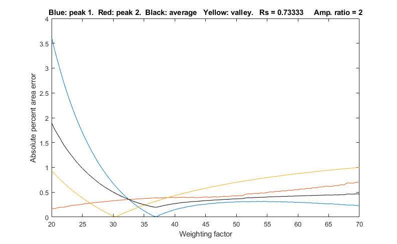 the errors of
measuring peak areas of two
overlapping Gaussians by the perpendicular drop
method using the autopeaks.m function.
It does this by applying different degrees of sharpening and
plotting the area errors (percent difference between the true and
measured errors) vs the sharpening factor, as shown on the right.
It also shows the height of the valley between the peaks (yellow
line). This demonstrates that (1) the optimum sharpening factor
depends upon the width and separation of the two peaks and on
their height ratio, (2) that the degree of sharpening is not
overly critical, often exhibiting a broad optimum region, (3) that
the optimum for the two peaks is not necessarily exactly the same,
and (4) that the optimum for area measurement usually does not
occur at the point where the valley is zero. (To run this script
you must have gaussian.m, derivxy.m, autopeaks.m,
val2ind.m, and halfwidth.m
in the path. Download these from https://terpconnect.umd.edu/~toh/spectrum/).
the errors of
measuring peak areas of two
overlapping Gaussians by the perpendicular drop
method using the autopeaks.m function.
It does this by applying different degrees of sharpening and
plotting the area errors (percent difference between the true and
measured errors) vs the sharpening factor, as shown on the right.
It also shows the height of the valley between the peaks (yellow
line). This demonstrates that (1) the optimum sharpening factor
depends upon the width and separation of the two peaks and on
their height ratio, (2) that the degree of sharpening is not
overly critical, often exhibiting a broad optimum region, (3) that
the optimum for the two peaks is not necessarily exactly the same,
and (4) that the optimum for area measurement usually does not
occur at the point where the valley is zero. (To run this script
you must have gaussian.m, derivxy.m, autopeaks.m,
val2ind.m, and halfwidth.m
in the path. Download these from https://terpconnect.umd.edu/~toh/spectrum/).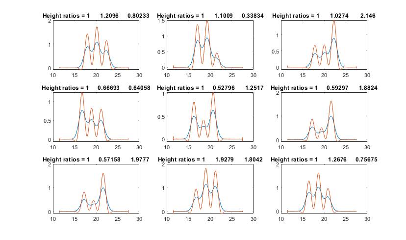 . A straight line is fit to the
calibration curve and the R2 is calculated, in order to demonstrate
(1) the linearity of the response, and (2) in independence of the
overlapping adjacent peaks. You can easily change:
. A straight line is fit to the
calibration curve and the R2 is calculated, in order to demonstrate
(1) the linearity of the response, and (2) in independence of the
overlapping adjacent peaks. You can easily change: values. (But this method does perform better than findpeaksG.m when
the peaks are noticeably asymmetric; see triangulationdemo for some examples). In contrast, measurepeaks.m makes no assumptions
about the shape of the peak.; it simply looks for the minima on
both sides of each peak to use as the dividing point between
peaks.
values. (But this method does perform better than findpeaksG.m when
the peaks are noticeably asymmetric; see triangulationdemo for some examples). In contrast, measurepeaks.m makes no assumptions
about the shape of the peak.; it simply looks for the minima on
both sides of each peak to use as the dividing point between
peaks. Peak area measurements by multiple
methods is a part of the Live Script Peak detection tool PeakDetection.mlx
described here
and illustrated on the left. This interactive tool allows optional
first-derivative
symmetrization of skewed peaks, as well as symmetrical
sharpening by Fourier
self-deconvolution, to enhance the resolution of overlapping
peaks and improve the accuracy of peak are measurement.
Peak area measurements by multiple
methods is a part of the Live Script Peak detection tool PeakDetection.mlx
described here
and illustrated on the left. This interactive tool allows optional
first-derivative
symmetrization of skewed peaks, as well as symmetrical
sharpening by Fourier
self-deconvolution, to enhance the resolution of overlapping
peaks and improve the accuracy of peak are measurement. 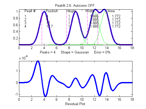


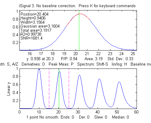

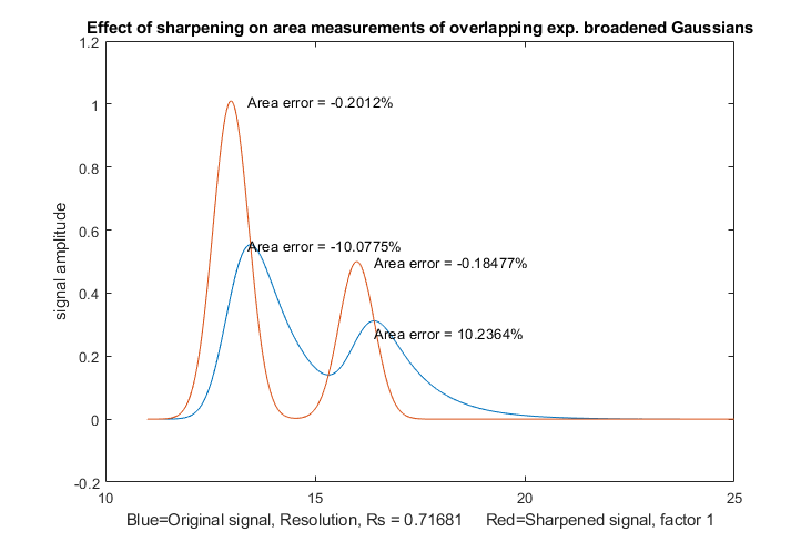 First-derivative symmetrization.
Although curve fitting is generally the most powerful method for
dealing with the combined effects of overlapping asymmetrical peaks
superimposed on an irrelevant background, the simpler technique of first derivative
sharpening can be useful as a method to reduce or eliminate
the effects of exponential broadening, resulting in a simpler shape
that is easier to fit. This is a simple techniques that calculates
the weighted sum of the original signal and its first derivative.
You just vary different first derivative weighting factor and choose
the one that makes the baseline after the peaks as low as possible
without going negative. As is the case with curve fitting, it's most
convenient is there is also isolated peak with the same exponential
broadening, because that peak can be used to determine more easily
the best value of the first derivative weighting factor.
First-derivative symmetrization.
Although curve fitting is generally the most powerful method for
dealing with the combined effects of overlapping asymmetrical peaks
superimposed on an irrelevant background, the simpler technique of first derivative
sharpening can be useful as a method to reduce or eliminate
the effects of exponential broadening, resulting in a simpler shape
that is easier to fit. This is a simple techniques that calculates
the weighted sum of the original signal and its first derivative.
You just vary different first derivative weighting factor and choose
the one that makes the baseline after the peaks as low as possible
without going negative. As is the case with curve fitting, it's most
convenient is there is also isolated peak with the same exponential
broadening, because that peak can be used to determine more easily
the best value of the first derivative weighting factor. 


