A common requirement
in scientific data processing is to detect peaks in a signal and
to measure their positions, heights, widths, and/or areas. One way
to do this is to make use of the fact that the first derivative of a peak has a
downward-going zero-crossing
at the peak maximum. But the presence of random noise in real
experimental signal will cause many false zero-crossing simply due
to the noise. To avoid this problem, the technique described here
first smooths the first derivative
of the signal, before looking for downward-going zero-crossings,
and then it takes only those zero crossings whose slope exceeds a
certain predetermined minimum (called the "slope threshold")
at a point where the original signal exceeds a certain minimum
(called the "amplitude threshold"). By carefully adjusting
the smooth width, slope threshold, and amplitude threshold, it's
possible to detect only the desired peaks and ignore peaks that
are too small, too wide, or too narrow. Moreover, this technique
can be extended to estimate the position, height, and width of
each peak by least-squares
curve-fitting of a segment of the original unsmoothed signal in the vicinity of
the zero-crossing. Thus, even if heavy smoothing of the first
derivative is necessary to provide reliable discrimination against
noise peaks, the peak parameters extracted by curve fitting are
not distorted by the smoothing, and
the effect of random noise in the signal is reduced by curve
fitting over multiple data points in the peak. This
technique is capable of measuring peak positions and heights quite
accurately, but the measurements of peak widths and areas is most
accurate if the peaks are Gaussian in shape (or Lorentzian, in the variant findpeaksL).
For the most accurate measurement of other peak shapes, or of
highly overlapped peaks, or of peak superimposed on a baseline,
the related functions findpeaksb.m,
findpeaksb3.m, findpeaksfit.m
utilize non-linear iterative curve
fitting with selectable peak shape models and baseline
correction modes.
The routine is now available in several different versions which
are described below:
(2) an interactive keypress-operated function,
called iPeak (ipeak.m), for adjusting the peak detection
criteria interactively to optimize for any particular peak type
(Matlab only). iPeak runs in the Figure window and use a simple
set of keystroke commands to reduce screen clutter, minimize
overhead, and maximize processing speed.
(3) A set of spreadsheets, available
in Excel and in OpenOffice formats.
(4) Real-time peak detection in
Matlab is discussed in Appendix
Y.
Simple fast functions for
detecting peaks in smooth or previously smoothed data.
allpeaks.m.allpeaks(x,y)Asuper-simplepeak
detector for x,y, data sets that lists everyyvalue that has loweryvalues on both sides. A related version, allpeaksw.m,
also estimates the width of the peaks, based upon the
assumption that the peaks are
locally Gaussian near the peak
tops. The variantallvalleys.mlists everyyvalue that hashigher yvalues on both sides. Type "help allpeaks" or "help
allpeaksw" for
an example.
peaksat.m. ("Peaks
Above Threshold") Syntax:P=peaksat(x,y,threshold).This function detects every y value that
(a) has lower y values on both sides and (b) is above
thespecifiedthreshold.Returns
a 2 bynmatrix
P with the x andy
values of each peak, wherenis
thenumberof detected
peaks. Type "help
peaksat"for
examples.
peaksatG.m.
("Peaks Above Threshold/Gaussian")
Syntax:P=peaksatG(x,y,threshold,peakgroup).This
function is similar to peakat.m
but it additionally performs a Gaussian
least-squares
fit to the top of each detected
peak to estimate its width and
area; the
number of data
points at the
top of the
peak that are
fit is determined
by the
input argument "peakgroup".
Returns a 5 bynmatrix
P with the x andy
values of each peak, wherenis
thenumberof
detected peaks. Type "help
peaksatG" for
examples.
These functions
do not have any internal smoothing. If the
data are noisy, smoothing should be applied
beforehand to prevent the detection of noise
peaks (see Smoothing). The
following functions, on the other hand,
apply internal smoothing before peaks
detection.
P=findpeaksx(x, y, SlopeThreshold, AmpThreshold, SmoothWidth,
PeakGroup, smoothtype)
P=findpeaksxw(x, y, SlopeThreshold, AmpThreshold, SmoothWidth,
PeakGroup, smoothtype)
Fast command-line functions to locate and count the positive
peaks in a noisy data sets. These functions detect peaks by
looking for downward zero-crossings in the smoothed first
derivative that exceed SlopeThreshold and peak amplitudes that
exceed AmpThreshold, and returns a list (in matrix P)
containing the peak number and the measured position and height of
each peak (and for the variant findpeaksxw,
the full
width at half maximum, determined by calling the halfwidth.m function) . It
can find and count over 10,000 peaks per second in very large
signals. The data are passed to the findpeaksx
function in the vectors x and y (x = independent variable, y =
dependent variable). The other parameters are user-adjustable:
SlopeThreshold
- Slope of the smoothed first-derivative that is taken to
indicate a peak. This discriminates on the basis of peak width.
Larger values of this parameter will neglect broad features of
the signal. A reasonable initial value for Gaussian peaks is
0.7*WidthPoints^-2, where WidthPoints is the number of data
points in the half-width (FWHM)
of the peak. AmpThreshold - Discriminates on the basis of peak height.
Any peaks with height less than this value are ignored. SmoothWidth - Width of the smooth function that is
applied to data before the slope is measured. Larger values of
SmoothWidth will neglect small, sharp features. A reasonable
value is typically about equal to 1/2 of the number of data
points in the half-width of the peaks. PeakGroup - The number of points around the "top part" of
the (unsmoothed) peak that are taken to estimate the peak
heights. If the value of PeakGroup is 1 or 2, the maximum y
value of the 1 or 2 points at the point of zero-crossing is
taken as the peak height value; if PeakGroup is n is 3
or greater, the average of the next n points is
taken as the peak height value. For spikes or very narrow peaks,
keep PeakGroup=1 or 2; for broad or noisy peaks, make PeakGroup
larger to reduce the effect of noise.
Smoothtype
determines the smoothing algorithm (see http://terpconnect.umd.edu/~toh/spectrum/Smoothing.html)
If smoothtype=1, rectangular (sliding-average
or boxcar)
If smoothtype=2, triangular (2 passes of
sliding-average)
If smoothtype=3, pseudo-Gaussian (3 passes of
sliding-average)
Basically, higher values yield greater reduction in
high-frequency noise, at the expense of slower execution. For a
comparison of these smoothing types, see SmoothingComparison.html.
The demonstration scriptsdemofindpeaksx.m and demofindpeaksxw.m finds,
numbers, plots, and measures noisy peaks with unknown random
positions. (Note that if two peaks overlap too much, the reported
width will be the width of the blended peak, in which cases it's
better to use findpeaksG.m, below).
Speed demonstration, comparing the peaksat.m and findpeaksx.m
functions, in Matlab 2020, on a Dell XPS i7 3.5Ghz
desktop. Note: Matlab's
tic" and "toc" functions are used to determine elapsed time.
Elapsed
time is 0.11, which is 110,000
peaks per second.
Functions for detecting and
measuring Gaussian peaks, findpeaksG.m,
or Lorentzian peaks, findpeaksL.m,
for Matlab or Octave.
P=findpeaksG(x, y, SlopeThreshold, AmpThreshold, SmoothWidth,
FitWidth, smoothtype)
P=findpeaksL(x, y, SlopeThreshold, AmpThreshold, SmoothWidth,
FitWidth, smoothtype) These functions locate the positive peaks in a noisy data
set, performs a least-squares
curve-fit of a Gaussian or Lorentzian function to
the top part of the peak, and computes the position, height,
and width (FWHM)
of each peak from that least-squares fit. (The 6th
input argument, FitWidth, is the number of data points around
each peak top that is fit). The other arguments are that same
as findpeaksx. Returns a list (in matrix P) containing the
peak number and the estimated position, height, width, and
area of each peak. It can find and curve-fit over 2800
peaks per second in very large signals. (This
is useful primarily for signals that have several data points in
each peak, not for spikes that have only one or two points, for
which findpeaksx is better).
The
function findpeaksplot.m
is a simple variant of findpeaksG.m that also
plots the x,y data and numbers the
peaks on the graph (if any are found). The
function findpeaksplotL.m
does the same thing optimized for Lorentzian
peak.
findpeaksSG.m
is a segmented variant of the findpeaksG function, with
the same syntax, except that the four peak detection parameters
can be vectors, dividing up the signal into regions that
are optimized for peaks of different widths. Any number of
segments can be declared, based on the length of the third
(SlopeThreshold) input argument. (Note: you only need
to enter vectors for those parameters that you want to vary
between segments; to allow any of the other peak detection
parameters to remain unchanged across all segments,
simply enter a single scalar value for that parameter;
only the SlopeThreshold must be a vector). The following example
declares two segments, with AmpThreshold remaining the same in
both segments:
FindpeaksSL.m
is the same thing for Lorentzian peaks.
A related function is findpeaksSGw.m
which is similar to the above except that is uses wavelet
denoising instead of
regular smoothing. It takes the wavelet level rather than
the smooth width as an input argument. The script TestPrecisionFindpeaksSGvsW.m
compares the precision and accuracy for peak position and
height measurement for both the findpeaksSG.m and
findpeaksSGw.m functions,
finding
that there is little to be gained in most cases by using the
wavelet denoise instead of smoothing. That is mainly because
in either case the peak parameter measurements are based on
least-squares fitting to the raw, not the smoothed,
data at each detected peak location, so the usual wavelet
denoising advantage of avoiding smoothing distortion does
not apply here.
In the graphic
example shown on the right, the demonstration scriptTestPrecisionFindpeaksSG.m
creates a noisy signal with three peaks of widely different
widths, detects and measures the peak positions, heights and
widths of each peak using findpeaksSG, then prints out the percent
relative standard deviations of parameters of the three peaks in
100 measurements with independent random noise. With 3-segment
peak detection parameters, findpeaksSG reliably detects and
accurately measures all three peaks. In contrast, findpeaksG,
tuned to the middle peak (using line 26 instead of line 25),
measures the first and last peaks poorly, because the peak
detection parameters are far from optimum for those peak widths.
You can also see that the precision of peak height
measurements gets progressively better (smaller relative
standard deviation) the larger the peak widths, simply
because there are more data points in wider peaks. (You
can change any of the variables in lines 10-18).
One difficulty
with the above peak finding functions it is annoying to have to
estimate the values of the peak
detection parameters that you need to use for your signals.
A quick way to estimate these is to use autofindpeaks.m,
which is similar to findpeaksG.m except that you can
optionally leave out the peak detection parameters and just
write "autofindpeaks(x, y)" or "autofindpeaks(x, y, n)",
where n is the "peak capacity", roughly the number of
peaks that would fit into that signal record (greater n
looks for many narrow peaks; smaller n looks for fewer
wider peaks and neglects the fine structure). Basically n
allows you to quickly adjust all of the peaks detection
parameters at once just by changing a single number. In
addition, if you do leave out the explicit peak detection
parameters, autofindpeaks will print out the numerical input
argument list that it uses in the command window, so you can
copy, paste, and edit for use with any of the findpeaks...
functions. If you call autofindpeaks with the output arguments
[P,A]=autofindpeaks(x,y,n), it returns the calculated peak
detection parameters as a 4-element row vector A, which you can
then pass on to other functions such as measurepeaks, effectively
giving that function the ability to calculate the peak detection parameters from a single
single number n. For example, a quick visual
estimate of the following signal indicates about 20 peaks, so you
use 20 as the third input argument:
Then you can use the values of the vector A as the peak detection
parameters for other peak detection functions, such as P=findpeaksG(x,y,A(1),A(2),A(3),A(4),1) or P=measurepeaks(x,y,A(1),A(2),A(3),A(4),1).
You will probably want to fine-tune the amplitude threshold A(2)
manually for your own needs.
Type "help autofindpeaks" and run the examples
there. autofindpeaksplot.m is
the same but also plots and numbers the peaks. The script testautofindpeaks.m runs all the
examples in the help file, plots the data and numbers the peaks
(like autofindpeaksplot.m), with a 1-second pause between each
example (animated graphic). Optimization of peak finding
Finding peaks in a signal depends on distinguishing
between legitimate peaks and other feature like noise and baseline
changes. Ideally, a peak detector should detect all the legitimate peaks and ignore all the
other features. This requires that a peak detector be "tuned" or
optimized for the desired peaks. For example, the Matlab/Octave
demonstration script OnePeakOrTwo.m
creates a signal (shown on the right)
that might be interpreted as either one peak at x=3 on a
curved baseline or as two peaks at x=.5
and x=3, depending on
context. The peak finding algorithms described here have input
arguments that allow some latitude for adjustment. In this
example script, the "SlopeThreshold" argument is adjusted to
detect just one or both of those peaks.
Similarly, the signal shown in the
figure on the left below could be interpreted as either as two
broad noisy peaks or as 25 little narrow peaks on
a two-humped background. The findpeaks... functions allow either
interpretation, depending in the peak detection parameters.
The optimum values of the input arguments for findpeaksG and
related functions depend on the signal and on which features of
the signal are important for your work. Rough values for these
parameters can be estimated based on the width of the peaks that
you wish to detect, as
described above, but for the greatest control it will be
best to fine-tune these parameters for your particular signal. A
simple way to do that is to use autopeakfindplot(x,
y, n) and adjust n until it finds the peak you
want; it will print out the
numerical input argument list so you can copy, paste, and edit
for use with any of the findpeaks... functions.
A more flexible way, if you are using Matlab, is to use the interactive
peak detector iPeak (described below),
which allows you to adjust all of these parameters individually by simple keypresses and displays the
results graphically and instantly. The script
FindpeaksComparison
shows how findpeakG compares to
the other peak detection functions
when applied
to a
computer-generated signal with
multiple peaks with variable types
and amounts of baseline and random
noise. By itself, autofindpeaks.m,
findpeaksG and findpeaksL do not
correct for a non-zero
baseline; if your
peaks are superimposed on a
baseline, you should subtract the
baseline first or use
the
other peak detection functions
that do correct for the baseline.
In the example shown on the left (using the interactive peak detector
iPeak program described below), suppose that
the important parts of the signal are two broad peaks
at x=4 and x=6, the second one half the
height of the first. The small jagged features are just random
noise. We want to detect the two peaks but ignore the noise. (The
detected peaks are numbered 1,2,3,...in the lower panel of this
graphic). This is what it looks like if the AmpThreshold
is too small or too large, if the
SlopeThreshold is too small or too large, if
the SmoothWidth is too small or too large, if
the FitWidth is too small or too large. If
these parameters are within the optimum range for this measurement
objective, the findpeaksG functions will return something like
this (although the exact values will vary with the noise and with
the value of FitWidth):
Peak# Position Height Width
Area 1 3.9649
0.99919 1.8237 1.94 2 5.8675
0.53817 1.6671 0.955 How is 'findpeaksG'
different from 'max' in Matlab or 'findpeaks' in the Signal
Processing Toolkit?
The 'max' function simply returns the largest single
value in a vector. Findpeaks
in the Signal Processing Toolbox can be used to find
the values and indices of all the peaks in a vector that are
higher than a specified peak height and are separated from their
neighbors by a specified minimum distance. My version of findpeaks
(findpeaksG) accepts both an
independent variable (x) and dependent variable (y) vectors, finds
the places where the average curvature over a specified region is
concave down, fits that region with a least-squares fit, and
returns the peak position (in x units), height, width, and area,
of any peak that exceeds a specified height. For example, let's
create a noisy series of peaks (plotted on the right) and apply both of these
findpeaks functions to the resulting data.
x=[0:.1:100]; y=5+5.*sin(x)+randn(size(x)); plot(x,y)
Now, most people just
looking at this plot of data would count 16 peaks, with
peak heights averaging about 10 units. Every time the statements
above are run, the random noise is different, but you would still
count the 16 peaks, because the signal-to-noise ratio is 10, which
is not that bad. But the findpeaks function in the Signal
Processing Toolbox,
[PKS,LOCS] = findpeaks(y,
'MINPEAKHEIGHT',5, 'MINPEAKDISTANCE', 11) counts anywhere from 11 to 20 peaks, with
an average height (PKS)
of 11.5.
In contrast, my findpeaksG function findpeaksG(x,y,0.001,5,11,11,3)counts
16 peaks every time, with an
average height of 10 plus or minus 0.3, which is much
more reasonable. It also measures the width and area, assuming the
peaks are Gaussian (or Lorentzian, in the variant findpeaksL). To
be fair, findpeaks
in the Signal Processing Toolbox, or my even faster
findpeaksx.m function, works better
for peaks that have only 1-3 data points on the peak; my
function is better for peaks that have more data points.
The demonstration script FindpeaksSpeedTest.m compares
the speed of the Signal Processing Toolkit (SPT) findpeaks,
peaksat, findpeaksx,
and findpeaksG
on the same large test signal with many peaks, updated for
Matlab 2020b running on a Dell XPS i7 3.5Ghz desktop: Number
Elapsed Peaks per Function of
peaks time second findpeaks (SPT)
160 0.012584 12715
peaksat
999 0.0012912 773699
findpeaksx
158 0.001444 109418
findpeaksG
157 0.011005 14267
findvalleys. There is also a
similar function for finding valleys
(minima), called findvalleys.m, which
works the same way as findpeaksG.m, except that it locates minima
instead of maxima. Only valleys above the
AmpThreshold (that is, more positive or less negative) are detected;
if you wish to detect valleys that have negative minima, then
AmpThreshold must be set more negative than that.
>> x=[0:.01:50];
y=cos(x);
P=findvalleys(x,y,0,-1,5,5) P =
1.0000 3.1416
-1.0000
2.3549
2.0000 9.4248
-1.0000
2.3549
3.0000 15.7080 -1.0000
2.3549
4.0000 21.9911 -1.0000
2.3549 .... The accuracy of the measurements of peak position,
height, width, and area by the findpeaksG function depends on the
shape of the peaks, the extent of peak overlap, the strength of
the background, and the signal-to-noise ratio. The width and area
measurements particularly are strongly influenced by peak overlap,
noise, and the choice of FitWidth. Isolated peaks of Gaussian
shape are measured most accurately. For peak of Lorentzian shape,
use findpeaksL.m
instead (the only difference is that the reported peak heights,
widths, and areas will be more accurate if the peak are actually
Lorentzian). See "ipeakdemo.m" below for an accuracy trial for
Gaussian peaks. For highly overlapping peaks that do not exhibit
distinct maxima, use peakfit.m or the Interactive Peak Fitter (ipf.m).
For
a direct comparison of the accuracy of findpeaksG vs
peakfit, run the demonstration script peakfitVSfindpeaks.m.
This script generates four very noisy peaks of different
heights and widths, then measures them in two different
ways: first with findpeaksG.m (figure on the left) and
then with peakfit.m, and
compares the results. The peaks detected by findpeaksG are
labeled "Peak 1", "Peak 2", etc. If you run this script
several times, it will generate the same peaks but with independent
samples of the random noise each time. You'll find
that both methods work well most of the time, with peakfit
giving smaller errors in most cases (because it uses all
the points in each peak, not just the top part), but
occasionally findpeaksG will miss the first (lowest) peak
and rarely it will detect an 5th peak that is not really
there. On the other hand, peakfit.m is constrained to fit
4 and only 4 peaks each time.
The
demonstration script FindpeaksComparison
compares the accuracy of
findpeaksG and findpeaksL
to several peak detection
functions when applied to
signals with multiple
peaks and variable types
and amounts of baseline
and random noise.
findpeaksb.mis a
variant of findpeaksG.m that more accurately measures peak
parameters by using iterative
least-square curve fitting based on my peakfit.m function
This yields better peak parameter values than findpeaksG
alone for three reasons:
(1) it can be set for
different peak shapes with the input argument
'PeakShape';
(2) it fits the entire peak,
not just the top part; and
(3) it has provision for background
subtraction (when the input argument "autozero" is set
to 1, 2, or 3 - linear, quadratic, or flat,
respectively).
This function works best with isolated
peaks that do not overlap. For version 3, the syntax is
P = findpeaksb(x,y, SlopeThreshold, AmpThreshold, smoothwidth,
peakgroup, smoothtype, windowspan, PeakShape, extra, AUTOZERO).
The first seven input arguments are exactly the same as
for the findpeaksG.m function; if you have been using
findpeaksG or iPeak to find and measure peaks in your
signals, you can use those same input argument values for
findpeaksb.m. The remaining four input arguments of are
for the peakfit function:
"windowspan" specifies
the number of data points over which each peak is fit
to the model shape (This is the hardest one to
estimate; in autozero modes 1 and 2, 'windowspan' must
be large enough to cover the entire single peak and
get down to the background on both sides of the peak,
but not so large as to overlap neighboring peaks);
"PeakShape" specifies
the model peak shape: 1=Gaussian, 2=Lorentzian, etc
(type 'help findpeaksb' for a list),
"extra" is the shape
modifier variable that is used for the Voigt, Pearson,
exponentially broadened Gaussian and Lorentzian,
Gaussian/Lorentzian blend, and bifurcated Gaussian and
Lorentzian shapes to fine-tune the peak shape;
"AUTOZERO"
is 0, 1, 2, or 3 for no, linear, quadratic, or flat
background subtraction.
The
peak table returned by this function has a
6th column listing the
percent fitting errors for each peak.
Here is a simple example with three Gaussians on a linear
background, comparing (a) plain findpeaksG,
to (b) findpeaksb without
background subtraction (AUTOZERO=0),
and to (c) findpeaksb with background subtraction
(AUTOZERO=1).
The demonstration script DemoFindPeaksb.m
shows how findpeaksb works with multiple
peaks on a curved background, and FindpeaksComparison
shows how findpeaksb compares to the
other peak detection functions when
applied to signals with multiple peaks
and variable types and amounts of
baseline and random noise.
findpeaksSb.mis a segmented
variant of findpeaksb.m. It has
the same syntax as findpeaksb.m,
except that the input arguments
SlopeThreshold, AmpThreshold,
smoothwidth, peakgroup, window, width,
PeakShape, extra, NumTrials, autozero,
and fixedparameters, can all
optionally be scalars or vectors with
one entry for each segment, in the
same manner as findpeaksSG.m.
Returns a matrix P listing the peak
number, position, height, width, area,
percent fitting error and "R2" of each
detected peak. In the example on the
right, the two peaks have the same
height above baseline (1.00) but
different shapes (the first Lorentzian
and the second Gaussian), very
different widths, and different
baselines. So, using findpeaksG or
findpeaksL or findpeaksb, it would be
impossible to find one set of input
arguments that would be optimum for
both peaks. But, using
findpeaksSb.m, different settings can
apply to different regions of the
signal. In this simple example, there
are only two segments,
defined by SlopeThreshold with 2
different values, and the other input
arguments are either the same or are
different in those two segments. The
result is that the peak height of the
both peaks is measured accurately.
SlopeThreshold=[.001
.00005];
AmpThreshold=.6;
smoothwidth=[5
120];
peakgroup=[5
120]; smoothtype=3;
window=[30
200];
PeakShape=[2
1]; extra=0;
NumTrials=1;
autozero=[3
0];
Peak #
Position
Height
Width Area
1
19.979
0.9882 1.487
1.565
2
79.805
1.0052 23.888
25.563
DemoFindPeaksSb.m
demonstrates the findpeaksSG.m
function by creating a random
number of Gaussian peaks whose
widths increase by a factor of
25-fold over the x-axis range and
that are superimposed on a curved
baseline with random white noise
that increases gradually; four
segments are used in this example,
changing the peak detection and
curve fitting values so that all
the peaks are measured accurately.
Graphic.
Printout.
findpeaksb3.m
is a more ambitious variant of findpeaksb.m that fits each
detected peak along with the previous and following peaks
found by findpeaksG.m, so as to deal better with overlap of
the adjacent overlapping peaks. The syntax is function FPB=findpeaksb3(x,y,
SlopeThreshold, AmpThreshold, smoothwidth, peakgroup,
smoothtype, PeakShape, extra, NumTrials, AUTOZERO, ShowPlots).
The demonstration script DemoFindPeaksb3.m shows
how findpeaksb3 works with irregular clusters of
overlapping Lorentzian peaks, as in the example on
the left (type "help findpeaksb3") for more.
The
demonstration
script FindpeaksComparison
shows how findpeaksb3 compares to the
other peak detection functions when
applied to signals with multiple peaks
and variable types and amounts of
baseline and random noise.
findpeaksfit.m is essentially a serial
combination of findpeaksG.m and peakfit.m. It uses the
number of peaks found and the peak positions and widths determined
by findpeaksG as input for the peakfit.m function, which then fits
the entire signal with the specified peak model. This
combination yields better values than findpeaksG alone, because
peakfit fits the entire peak, not just the top part, and it deals
with non-Gaussian and overlapped peaks. However, it fits only
those peaks that are found by findpeaksG. The syntax is
function [P,FitResults,LowestError,BestStart,xi,yi] =
findpeaksfit(x, y, SlopeThreshold, AmpThreshold, smoothwidth,
peakgroup, smoothtype, peakshape, extra, NumTrials, autozero,
fixedparameters, plots)
The first
seven input arguments are exactly the same as for the findpeaksG.m
function; if you have been using findpeaksG
or iPeak to find and measure peaks in your
signals, you can use those same input argument values for
findpeaksfit.m. The remaining six input arguments of
findpeaksfit.m are for the peakfit
function; if you have been using peakfit.m or ipf.m
to fit the peaks in your signals, then you can use those same
input argument values for findpeaksfit.m.
The
demonstration script findpeaksfitdemo.m,
shows findpeaksfit automatically finding and fitting the peaks in
a set of 150 signals, each of which may have 1 to 3 noisy
Lorentzian peaks in variable locations, artificially slowed
down with the "pause" function so you can see it better.
Requires the findpeaksfit.m and lorentzian.m functions installed. This
script was used to generate the GIF animation shown on the left.
Type "help findpeaksfit" for more information.
Which to use: findpeaksG/L,
findpeaksb, findpeaksb3, or findpeaksfit? The demonstration
script FindpeaksComparison.m
compares the peak parameter accuracy all four of those peak
detection functions applied to a computer-generated signal with
multiple peaks plus variable types and amounts of
baseline and random noise. (Requires those four functions, plus
gaussian.m, lorentzian.m, modelpeaks.m, findpeaksG.m,
findpeaksL.m, pinknoise.m, and propnoise.m, in the Matlab/Octave
path). Results are displayed graphically in figure windows 1, 2, and 3 and printed out in a table of
parameter accuracy and elapsed time for each method, as shown
below. You may change the lines in the script marked
by <<< to modify the number and character and amplitude
of the signal peaks, baseline, and noise. Make the signal
similar to yours to discover which method works best for your type
of signal. The best method depends mainly on the shape and
amplitude of the baseline and on the extent of peak overlap. Type
"help FindpeaksComparison"
for details. (Times updated for Matlab 2020 on
Dell XPS i7
3.5Ghz).
Average absolute
percent errors of all peaks
Position Height Width Elapsed
error error
error
time, sec findpeaksG 0.35955
38.5733 25.7977 0.005768 findpeaksb 0.388283
8.5024 14.3295 0.069061 findpeaksb3 0.27187
3.7445 3.0474 0.49538
findpeaksfit 0.519302
8.0417 24.035 0.273
Note: findpeaksfit.m differs from findpeaksb.m
in that findpeaksfit.m fits all the found
peaks at one time with a single multi-peak model, whereas findpeaksb.mfits each peak separately with a single-peak model, and
findpeaksb3.m
fits each detected peak along with the previous
and following peaks. As a result, findpeaksfit.m works better with a
relatively small number of peak that all overlap, whereas findpeaksb.m
works better with a large number of isolated non-overlapping
peaks, and findpeaksb3.m works for large
numbers of peaks that overlap at most one or two adjacent
peaks. FindpeaksG/L is simple and fast, but it does
not perform baseline correction; findpeaksfit
can perform flat, linear, or quadratic baseline
correction, but it works only over the entire signal at once;
in contrast, findpeaksb and findpeaksb3 perform local baseline
correction, which often works well if the baseline is curved
or irregular.
Other related functions findpeaksG2d.m
is a variant of findpeaksSG that can be used to locate the
positive peaks and shoulders in a noisy x-y time series
data set. Detects peaks in the negative of the second
derivative of the signal, by looking for downward slopes in
the third derivative that exceed SlopeThreshold. See TestFindpeaksG2d.m.
[M,A]=autopeaks.m
is a peak detector for peaks of arbitrary shape; it's basically a
combination or autofindpeaks.m and
measurepeaks.m. It has similar syntax
to measurepeaks.m, except that the
peak detection parameters (SlopeThreshold, AmpThreshold,
smoothwidth peakgroup, and smoothtype) can be omitted and
the function will calculate trial values in the manner of autofindpeaks.m. Using the simple
syntax [M,A]=autopeaks(x, y) works well in some cases, but if not
try [M,A]=autopeaks(x, y, n), using different values of n (roughly
the number of peaks that would fit into the signal record)
until it detects the peaks that you want to measure. Like
measurepeaks, it returns a table M containing the peak number,
peak position, absolute peak height, peak-valley difference,
perpendicular drop area, and tangent skim area of each peak it
detects, but is also can optionally return a vector A containing
the peak detection parameters that it calculates (for use by other
peak detection and fitting functions). For the most precise
control over peak detection, you can specify all the peak
detection parameters by typing M=autopeaks(x,y, SlopeThreshold,
AmpThreshold, smoothwidth, peakgroup). [M,A]=autopeaksplot.m
is the same but it also plots the signal and the individual peaks
in the manner of measurepeaks.m (shown above). The script testautopeaks.m runs all the examples
in the autopeaks help file, with a 1-second pause between each
one, printing out results in the command window and additionally
plotting and numbering the peaks (Figure window 1) and each
individual peak (Figure window 2); it requires gaussian.m and fastsmooth.m
in the path.
The function peakstats.m uses the same
algorithm as findpeaksG, but it computes and
returns a table of summary statistics of the
peak intervals (the x-axis interval between
adjacent detected peaks), heights, widths, and
areas, listing the maximum, minimum, average, and
percent standard deviation of each, and optionally
plotting the x,y data with numbered peaks in
figure window 1, printing the table of peak
statistics in the command window, and plotting the
histograms
of the peak intervals, heights, widths, and areas
in the four quadrants of figure window 2. Type
"help peakstats". The syntax is the same as
findpeaksG, with the addition of a 8th input
argument to control the display and plotting. Version
2, March 2016, adds median and mode. Example:
x=[0:.1:1000];
y=5+5.*cos(x)+randn(size(x));
PS=peakstats(x,y,0,-1,15,23,3,1);
Peak Summary Statistics
158 peaks detected
Interval Height
Width Area
Maximum 6.6428
10.9101 5.6258 56.8416
Minimum 6.0035
9.1217 2.5063 28.2559
Mean
6.283 9.9973
3.3453 35.4737
% STD
1.8259 3.4265
15.101 12.6203
Median
6.2719 10.026 3.2468
34.6473
Mode
6.0035 9.1217
2.5063 28.2559
With the last input argument omitted or
equal to zero, the plotting and printing in the
command window are omitted; the numerical values
of the peak statistics table are returned as a 4x4
array, in the same order as the example above.
tablestats.m (PS=tablestats(P,displayit))
is similar to peakstats.m except that it accepts
as input a peak table P such as generated by
findpeaksG.m, findvalleys.m, findpeaksL.m,
findpeaksb.m, findpeaksplot.m, findpeaksnr.m,
findpeaksGSS.m, findpeaksLSS.m, or findpeaksfit.m
- any of the functions that return a table of
peaks with at least 4 columns listing peak number,
height, width, and area. Computes the peak
intervals (the x-axis interval between adjacent
detected peaks) and the maximum, minimum, average,
and percent standard deviation of each, and
optionally displaying the histograms of the peak
intervals, heights, widths, and areas in figure
window 2. Set the optional last argument displayit
= 1 if the histograms are to be displayed,
otherwise not. Example:
FindpeaksE.m
is a variant of findpeaksG.m that additionally
estimates the percent relative fitting error of
each peak (assuming a Gaussian peak shape) and
returns it in the 6th column of the peak
table.
Example:
Peak
start and end. Defining the
"start" and "end" of the peak (the x-values where the peak
begins and ends) is a bit arbitrary because typical peak
shapes approach the baseline asymptotically far from the peak
maximum. You might define the peak start and end points as the
x values where the y value is some small fraction, say 1%, of
the peak height, but then the random noise on the baseline is
likely to be a large fraction of the signal amplitude at that
point. Smoothing to reduce noise is likely to distort and
broaden peaks, effectively changing their start and end
points. Overlap of peaks also greatly complicates the issue.
One solution is to fit each peak
to a model shape, then calculate the peak start and end
from the model expression. That method minimizes the noise
problem by fitting the data over the entire peak, and it can
handle overlapping peaks, but it works only if the peaks can
be modeled by available fitting programs. For example,
Gaussian peaks can
be shown to reach a fraction a of the
peak height at x = p + or - sqrt(w^2 log(1/a))/(2
sqrt(log(2))) where p is the peak position and w
is the peak width (full width at half maximum). So, for
example if a= .01, x = p+
or -w*sqrt((log(2)+log(5))/(2
log(2))) = 1.288784*w. Lorentzian peaks can
be shown to reach a fraction a of the
peak height at x = p+
or -sqrt[(w^2 - aw^2)/a]/2. If a = .01, x = p+
or -(3/2 sqrt(11)*w) =
4.97493*w. The findpeaksG variants findpeaksGSS.m and findpeaksLSS.m, for Gaussian
and Lorentzian peaks respectively, compute the peak start and
end positions in this manner and return them in the 6th and
7th columns of the peak table P.
The problem with this method
is that it requires an analytical peak model, expressed as a
closed-form expression, that can be solved algebraically for
their start and end points. A more versatile method is to fit
a model to the peak data by iterative
curve fitting, and then use the best-fit model to locate
the start and stop points by interpolation. For complex peak
shapes, the model need not be limited to a single peak;
very often complex peak shapes can be modeled as the sum of
simple shapes, such as Gaussians. An example of this method is
demonstrated in the script StartAndEnd.m,
which simulates a noisy, asymmetrical peak and then applies
this method using the downloadable peakfit.m
function. You can select the start/stop cut-off point as a
fraction of the peak height in line 8 and the amount or random
noise in line 7. The default for both values is 0.01 (or 1%),
which means that, at the cut-off points, the signal-to-noise
ratio is very poor. Nevertheless, the start and end points can
be calculated surprisingly precisely, because they are
calculated from the best-fit model (contained in the output
arguments xi and yi of the peakfit function), which averages
out the noise over the entire signal (the more data points the
better). The animation on the left shows the method in
operation for 50 repeat measurements with different random
noise samples, first with 1% noise and then with 10% noise.
Despite the poor signal-to-noise ratio at the cut-off points,
the relative standard deviation of the measured start and end
times (marked by the vertical lines) is only about 0.2%. (Even
when the noise is increased 10-fold to 0.1 in line 7, the
results are still surprisingly good).
findpeaksT.mand
findpeaksTplot.m are
variants of findpeaksG that measure the peak parameters by automatically
constructing a triangle around each peak with its sides
tangent to the sides of the peak, as shown on the right (script that generated this graphic).
This method mimics the geometric construction method that was
formerly used to measure peak parameters manually before the
age of computers. Peak height is taken as the apex of the
triangle, which is slightly higher than the peak of the
underlying curve. The performance of this method is poor when
the signals are very noisy or if the peaks overlap, but in a
few circumstances the triangle construction
method might be more accurate for the measurement of
peak area than the Gaussian method, especially if the peaks
are asymmetric or of uncertain shape (see the
demo function triangulationdemo.m
for some examples: click for
graphic).
findsteps.m, syntax:
P=findpulses(x, y, SlopeThreshold, AmpThreshold, SmoothWidth,
peakgroup), locates positive transient steps in noisy x-y time
series data, by computing the first derivative of y that exceed
SlopeThreshold, computes the step height as the difference between
the maximum and minimum y values over a number of data point equal
to "Peakgroup". Returns list (P) with step number, x position, y
position, and the step height of each step detected;
"SlopeThreshold" and "AmpThreshold" control step sensitivity;
higher values will neglect smaller features.
Increasing "SmoothWidth" reduces small sharp false steps caused by
random noise or by "glitches" in the data acquisition. See findsteps.png for a real example. And findstepsplot.m plots the signal and
numbers the peaks. Rectangular
pulses (square waves) require a different approach, based
on amplitude discrimination rather than differentiation. The
function "findsquarepulse.m"
(syntax S=findsquarepulse(t,y,threshold) locates the
rectangular pulses in the signal t,y that exceed a y-value of
"threshold" and determines their start time, average height
(relative to the baseline) and width. DemoFindsquare.m creates a test signal
(with a true height of 2636 and a height of 750) and calls findsquarepulse.m
to demonstrate. If the signal is very noisy, some preliminary
rectangular smoothing (e.g. using fastsmooth.m) before calling
findsquarepulse.m may be helpful to eliminate false peaks.
NumAT(m,threshold):
"Numbers Above Threshold": Counts the
number of adjacent elements in the vector 'm' that are greater
than or equal to the scalar value 'threshold'. Returns a matrix
listing each group of adjacent values, their starting index, the
number of elements in each group, the sum of each group, and the
average (mean) of each group. Type "help NumAT" and try
the example.
Using
the peak table
All these peak finding functions return a peak table as a matrix,
with one row for each peak detected and with several columns
listing, for example, the peak number, position, height, width,
and area in columns 1 - 5 (with additional columns included for
the variants measurepeaks.m, findpeaksnr.m, findpeaksGSS.m, and findpeaksLSS.m). You
can assign this matrix to a variable (e.g. P, in the
examples above) and then use Matlab/Octave notation
and built-in functions to extract specific information from that
matrix. The powerful combination of functions and matrix/vector
"colon" notation allows you to construct compact expressions
that extract the very specific information that you need.
For example:
[P(:,2) P(:,3)]is the time
series of peak heights (peak position in the first column and peak
height in the second column) mean(P(:,3))
returns the average peak height of all peaks (because
peak height is in column 3). Also works with median.
max(P(:,3))
returns the maximum peak height. Also
works with min. hist(P(:,3))
displays the histogram of peak heights. std(P(:,4))./mean(P(:,4))
returns the relative standard deviation of the peak widths (column
4). P(:,3)./max(P(:,3)) returns the
ratio of each peak height (column 3)
to the height of the highest peak detected. 100.*P(:,5)./sum(P(:,5)) returns the percentage
of each peak area (column 5)
of the total area of all peaks detected.
sortrows(P,2) sorts P by peak
position; sortrows(P,3) sorts P by peak
height (smallest to largest).
To create "d" as the vector of x-axis
(position) differences between adjacent peaks (because peak
position is in column 2).
for
n=1:length(P)-1;d(n)=max(P(n+1,2)-P(n,2));end
(In
Matlab/Octave, multiple statements can be placed on one line,
separated by semicolons.)
The downloadable function [index,closestval]
= val2ind(v,val)
returns the index and the value of the element of vector 'v' that
is closest to 'val' (download this function and place in the
Matlab path). It's very useful in working with peak tables: val2ind(P(:,3),7.5)
returns the peak number of the peak whose height (column
3) is closest to 7.5 P(val2ind(P(:,2),7.5),3) returns
the peak height (column 3) of the peak whose position (column
2) is closest to 7.5 P(val2ind(P(:,3),max(P(:,3))),:) returns the row
vector of peak parameters of the highest peak in peak
table P.
The three statements j=P(:,4)<5.8;k=val2ind(j,1);P(k,:)
return the matrix of peak parameters of all peaks in P
whose widths (column 4) are less than 5.8.
Finding peaks in multi-column data. The script FindingPeaksInMultiColumnData.m
shows how to read a multi-column dataset from an Excel
file and detect the peaks in each column, returning the
peak data in a 3-dimentional table of results PP.
DemoFindPeak.m
is a simple demonstration script using the findpeaksG function on noisy
synthetic data. Numbers the peaks and prints out the peak table
in the Matlab command window:
DemoFindPeakSNR is a
variant of DemoFindPeak.m that uses findpeaksnr.m to compute the
signal-to-noise ratio (SNR) of each peak and returns it in the 5th
column (click
for graphic).
DemoFindPeaksb.mis
a similar demonstration script that uses thefindpeaksbfunction
on noisy synthetic data consisting of variable numbers of
Gaussian peaks superimposed on a variable curved
background. (The findpeaksG function would not give
accurate measurements of peak height, width, and area for this
signal, because it does not correct for the background). Relative Percent Errors Position
Height Width Area
-0.00224 0.54487
1.4057 1.9429
-0.02727 5.0091
8.9204 13.483
0.008429 -1.1224 -1.4923
-2.6315
....
% Root mean square errors
ans =
0.044428 2.2571
3.8253 5.8501
Peak Identification
The command line function idpeaks.m is
used for identifying peaks according to their x-axis maximum
positions, which is very useful in spectroscopy and in
chromatography. The syntax is
It finds peaks in the signal "DataMatrix" (x-values in column 1
and y-values in column 2), according to the peak detection
parameters "AmpT", "SlopeT", "SmoothWidth", "FitWidth" (see the
"findpeaksG" function above), then compares the found peak
positions (x-values) to a database of known peaks, in the form of
an array of known peak maximum positions ('Positions') and
matching cell array of names ('Names'). If the position of a peak
found in the signal is closer to one of the
known peaks by less than the specified maximum error ('maxerror'),
that peak is considered a match and its peak position, name,
error, and peak amplitude (height) are entered into the output
cell array "IdentifiedPeaks". The full list of detected peaks,
identified or not, is returned in "AllPeaks". Use "cell2mat" to
access numeric elements of IdentifiedPeaks,e.g. cell2mat(IdentifiedPeaks(2,1))
returns the position of the first identified peak, cell2mat(IdentifiedPeaks(2,2))
returns its name, etc. Obviously for your own applications, it's up to you to
provide your own array of known peak maximum positions
('Positions') and matching cell array of names ('Names') for
your particular types of signals. The related function idpeaktable.m
does the same thing for a peak table P returned by any of my peak finder
or peak fitting functions, having one row for each peak and
columns for peak number, position, and height as the first three
columns. The syntax is [IdentifiedPeaks] =
idpeaktable(P,maxerror,Positions,Names). The
interactive iPeak function described in
the next section has this function built inas one
of the keystroke commands.
Example: Download idpeaks.zip, extract it, and place the
extracted files in the Matlab or Octave path.
This contains a high-resolution atomic emission spectrum of copper
('spectrum', x = wavelength in nanometers; y = amplitude) and a
data table of known Cu I and Cu II atomic lines ('DataTable')
containing the positions and names of many copper lines. The
idpeaks function detects and measures the peak locations of all
the peaks in "spectrum", then looks in 'DataTable' to
see if any of those peaks are within .01 nm of any entry in the
table and prints out the peaks that match.
ans= 'Position' 'Name' 'Error' 'Amplitude' [221.02] 'Cu II 221.027' [ -0.0025773] [ 0.019536] [221.46] 'Cu I 221.458' [ -0.0014301] [ 0.4615] [221.56] 'Cu I 221.565' [-0.00093125] [ 0.13191] .................... etc...
Peak detection tool
PeakDetection.mlx
is an interactive Live Script for peak detection and
measurement. It collects into one easy-to-use tool several of the
functions previously described, including a selection of peak
detectors, data smoothing, symmetrization, peak sharpening, and
curve fitting, with interactive sliders and drop-down menus
to control them interactively.
Clicking the OpenDataFile button in line
1 opens up a file browser, allowing you to navigate to your
data file (in .csv or .xlsx format).
The startpc and endpc sliders in lines 5 and
6 allow you to set the start and end of the region to focus on
(expressed as a percentage of the total data length).
You can choose a peak detector using the PeakDetector drop-down
menu in line 20.
The ListPeaks and LabelPeaks check boxes in
lines 3 and 4 allow you to number the peaks on the graph
and/or to display a list of peak parameters of the detected
peaks.
You can optionally try to sharpen the peaks,
to enable detection of weak side peak or shoulders, by
clicking the SharpenPeaks check box in line 13.
You can also apply iterative least-square curve
fitting, by clicking the FitDetectedPeaks check
box on line 26. and selecting the desired fitting function
shape from the PeakShape drop-down menu on line 27.
The position and width of the peaks estimated by the peak
detectors is used as the first-guess starting point for the
iterative fit; therefore only detected peaks will be
included in the fit. This function requires that peakfit.m be in
the Matlab path. (Generally, curve fitting is best applied only
to the unsmoothed data; however, if peak
sharpening or symmetrization is applied (line 9 or 13), it
uses the processed data).
The function of each of the controls is described in the
associated comment lines. For examples of this tool's
application to several different kinds of widely varying peak
data, see the PDF file PeakDetector.pdf, which
references a set of .csv data files which as also downloadable
from the same address.
(To see the graphs on the right as above, right-click on the
right panel and select "Disable synchronous scrolling").
iPeak is a
keyboard-operated
interactive peak finder for time series data, based on the "findpeaksG.m" and"findpeaksL.m"
functions, for Matlab only.Its
basic operation is similar to iSignaland ipf.m.
(If
you are using Octave instead of Matlab, there is a separate Octave version, which
uses different keys for pan and zoom). Press the K key
to list the keystroke commands. It accepts data in a single
vector, a pair of vectors, or a matrix with the independent
variable in the first column and the dependent variable in the
second column. If
you call iPeak with only those one or two input
arguments, it estimates a default initial value for the peak
detection parameters (AmpThreshold, SlopeThreshold, SmoothWidth, and FitWidth)based on the formulas
below and
displays those values at the bottom of the screen.
WidthPoints=length(y)/20;
SlopeThreshold=WidthPoints^-2;
AmpThreshold=abs(min(y)+0.1*(max(y)-min(y)));
SmoothWidth=round(WidthPoints/3);
FitWidth=round(WidthPoints/3);
You can then fine-tune the peak
detection by using the A/Z, S/X,
D/C, and F/V keys.
Recent additions: Added mode(y) subtraction as the 4th
baseline correction mode selected by the T key. Previous
version added measUrepeaks function (Shift-U) to
display perpendicular drop and tangent skim area measurements.
Added Shift-Y to enter de-tailing (sYmmetrization)
factor for exponentially modified peaks, and 1 & 2 (and Shift-1
& Shift-2) to adjust.
Example 1:One input argument; data in single vector: >>
y=cos(.1:.1:100);ipeak(y)
Example 2: One input argument; data in two columns of a matrix:
>> x=[0:.01:5]';y=x.*sin(x.^2).^2;M=[x
y];ipeak(M)
Example 3: Two input
arguments; data in separate x and y vectors: >> x=[0:.1:100];y=(x.*sin(x)).^2;ipeak(x,y);
Example 4: When you start iPeak using the simple
syntax above, the initial values of the peak detection
parameters are calculated as described above,but if it starts off by picking up
far too many or too few peaks, you can add an additional input
argument (after the data) to control peak sensitivity.
>> x=[0:.1:100];
y=5+5.*cos(x)+randn(size(x));
ipeak(x,y,10); or
>> ipeak([x;y],10); or
>> ipeak(humps(0:.01:2),3)
or >> x=[0:.1:10];
y=exp(-(x-5).^2);
ipeak([x' y'],1)
The additional numeric argument is an estimate of maximum
peak density(PeakD), the ratio
of the typical peak width to the length of the entire data
record. Small values detect fewer peaks; larger values detect more peaks. It effects only the
starting values for
the peak detection parameters. (It's just a quick way to set
reasonable initial values of the peak detection parameters, so you won't have so much adjusting
to do).
>> load sunspots >> ipeak(year,number,20)
Peaks in annual sunspot numbers from 1700 to 2009
(download the datafile).
Sunspot data downloaded
from NOAA,
iPeak displays the
entire signal in the lower half of the Figure window and an
adjustable zoomed-in section in the upper window. Pan and zoom
the portion in the upper window using the cursor arrow
keys. The
peak closest to the center of the upper window is labeled in the
upper left of the top window, and it peak position, height, and
width are listed. The Spacebar/Tab keysjump to the next/previous detected
peak and displays it in the upper window at the current zoom
setting (use
the up and down cursor arrow keys to adjust the zoom range). Or you can pressthe J key to jump to a specified peak
number.
Adjust the peak detection
parameters AmpThreshold (A/Z keys), SlopeThreshold (S/X), SmoothWidth
(D/C), FitWidth (F/V) so that it detects the
desired peaks and ignores those that are too small, too broad,
or too narrow to be of interest. You can also type in a specific value of
AmpThreshold by pressing Shift-A or a specific value of
SlopeThreshold by pressing Shift-S. Detected peaks are numbered from
left to right.
Press P to display the peak table of all the detected
peaks and their measurements by peak-top curve fitting (Peak #,
Position, Height, Width, Area, and percent fitting error):
Gaussian shape mode (press Shift-G to change) Window span: 169 units Linear baseline subtraction Peak# Position Height
Width Area Error 1 500.93
6.0585 34.446 222.17 9.573 2 767.75
1.8841 105.58 211.77 25.979 3
1012.8 0.2015 35.914
7.7 269.21 4...........
Press Shift-U to measure the peaks by the
perpendicular drop and tangent skim methods:
Peak Area Measurement (Shift-U
key)
Peak Position PeakMax Peak-valley Perp drop Tan skim
1 300.19 12.011
9.3502 839.32 537.85
2 399.84 10.011
6.8604 700.83 363.15 3 498.67
1.9994 0.85312
125.29 31.4 4
............
Press Shift-G to cycle between
Gaussian, Lorentzian, and flat-top shape modes. Press Shift-P
to save peak table as disc file. Press U to switch
between peak and valley mode. Don't forget that only valleys above (that is,
more positive or less negative than) the AmpThreshold are
detected; if you wish to detect valleys that have negative
minima, then AmpThreshold must be set more negative than
that. Note: to speed up the operation for
signals over 100,000 points in length, the lower window is
refreshed only when the number of detected peaks changes or if
the Enter key is pressed. Press K to see all
the keystroke commands.
Press U key to switch
between peak and valley mode.
If the density of data points on the peaks is too low
- less than about 4 points - the peaks may not be reliably
detected; you can improve reliability by using the
interpolation command (Shift-I) to re-sample the data
by linear interpolation to a larger number of
points. Conversely, if the density of data
points on the peaks of interest is very high - say, more than
100 points per peak - then you can speed up the operation of
iPeak by re-sampling to a smaller number
of points.
Peak
Summary Statistics.The E key prints a table
of summary statistics of the peak intervals (the x-axis
interval between adjacent detected peaks), heights, widths,
and areas, listing the maximum, minimum, average,
and percent standard deviation, and displaying the histogramsof the peak intervals, heights,
widths, and areas in figure window 2. Peak
Summary Statistics
149 peaks detected
No baseline correction
Interval Height Width Area
Maximum 1.3204 232.772
0.3340 80.7861
Minimum 1.1225 208.058
0.2714 61.6991
Mean
1.2111 223.368 0.3131 74.4764
% STD 2.8931
1.9115 3.091 4.0858
Example
5: Six
input arguments. As above, but input arguments 3 to 6 directly
specifies initial values of AmpThreshold (AmpT), SlopeThreshold (SlopeT), SmoothWidth (SmoothW), FitWidth (FitW). PeakD is ignored in this case, so
just type a '0' as the second argument after the data matrix). >>
ipeak(datamatrix,0,.5,.0001,20,20);
Pressing 'L' toggles ON and OFF the peak labels in the
upper window.
Keystrokes allow you to pan
and zoom the upper window, to inspect each peak in detail if
desired. You
can set the initial values of pan and zoom in optional input
arguments 7
('xcenter') and
8 ('xrange'). See example 6 below.
The Y keytoggles between linear and log
y-axis scale in the lower window (a log axis is good for
inspecting signals with high dynamic range).It effects only the lower window
display and has no effect on the data itself or on the peak detection and measurements.
The Y key displays the signal on a Log
scale in the lower window, which makes the
smaller peaks easier to see.
Example 6: Eight input arguments. As above, but input arguments 7 and 8 specify the initial pan and zoom settings, 'xcenter' and 'xrange', respectively. In this example, the x-axis data
are wavelengths in nanometers (nm), and the upper window zooms in on a very
small0.4 nm region centered on 249.7 nm.
(These data,
provided in the ZIP file, are from a
high-resolution atomic spectrum).
>> load
ipeakdata.mat >> ipeak(Sample1,0,100,0.05,3,4,249.7,0.4); Baseline correction methods.The T key
cycles the baseline correction mode from off, linear,
quadratic, flat, linear mode(y), flat
mode(y), and then back to off. The current mode is
displayed above the upper panel. When the
baseline correction is OFF, peak heights are measured relative
to zero. (Use this method
mode when the baseline is zero or if you have
previously subtracted the baseline from the entire signal using the Bkey). In thelinear orquadraticmethods, peak heights are automatically
measured relative to the local baseline interpolated from the points at the ends of the
segment displayed in the upper panel; use the zoom controls to isolate a group of peaks so that the signal returns to the
local baseline at
the beginning and end
of the segment
displayed in the upper window. The peak heights, widths, and areas in the peak table (R or P keys)will be automatically corrected for the baseline.The linear orquadratic methods will work best if the peaks are well separated so
that the signal returns to the local baseline between the
peaks. (If the peaks are highly overlapped, or if they are not
Gaussian in shape, the best results will be obtained by using
the curve fitting function - the N or M keys. The 3rd method flat is used only for curve fitting
function, to account
for a flat baseline offset without reference to the edges
of the signal segment being fit).
The mode(y)
methods 4 and 5 subtract the most common y value (the
statistical "mode") from all the points in the selected region.
For peak-type signals where the peaks often return to the baseline
between peaks, the most common value is usually a good
approximation of the baseline even if the signal does not return
to the baseline at the ends as required by methods 2 and 3 (graphic example).
Example 7: Nine input arguments. As example 6, but the 9th
input argument sets
the background correction mode (equivalent to pressing the T key)'
0=OFF; 1=linear; 2=quadratic, 3=flat, 4=mode(y). If not
specified, itis initially OFF. >> ipeak(Sample1,0,100,0.00,3,4,249.7,0.4,1);
Converting to command-line functions. To aid in
writing your own scripts and function to automate processing, the
'Q' key prints out the findpeaksG, findpeaksb, and
findpeaksfit commands for the segment of the signal in the upper
window and for the entire signal, with most or all of the input
arguments in place, so you can Copy and Paste into your own
scripts. The 'W' key similarly prints out the peakfit and
ipf commands. This provides a way to deal with signals
that require different signal processing in different regions of
their x-axis ranges, by allowing you to create a series of
command-line functions for each local region that, when executed
in sequence, quickly process each segment of the signal
appropriately.
Shift-Ctrl-S transfers the current signal to iSignal.m
and Shift-Ctrl-P transfers the current signal to
Interactive Peak Detector (iPeak.m), if those functions
are installed in your Matlab path.
Ensemble averaging.
For signals that contain repetitive waveform patterns occurring in
one continuous signal, with nominally the same shape except for
noise, the ensemble averaging function (Shift-E) can
compute the average of all the repeating waveforms. It works by
detecting a single peak in each repeat waveform in order to
synchronize the repeats (and therefore does not require that the
repeats be equally spaced or synchronized to an external reference
signal). To use this function, first adjust the peak detection
controls to detect only one peak in each repeat pattern,
then zoom in to isolate any one of those repeat patterns, and then
press Shift-E. The average waveform is displayed in Figure
2 and saved as "EnsembleAverage.mat" in the current directory.See iPeakEnsembleAverageDemo.m.
De-tailing peaks with
exponential tails. If your signal has peaks tail
that to the right or left because they have been
exponentially broadened, you can remove the tails by the
first-derivative
addition technique described previously. To activate
this process, press Shift-Y, enter a rough estimate
of the exponential time constant, and then use the 1
and 2 keys to adjust the de-tailing factor by 10%
(or Shift-1 and Shift-2 to adjust by 1%). Increase the factor
until the baseline after the peak goes negative, then
increase it slightly so that it is as low as possible
but not negative. (It the peaks tail to the left
rather than the right, use a negative factor). This
results in narrower, taller peaks, and it works with any
peak shape that has been exponentially broadened. It has the
same effect as deconvoluting the exponential function from
the broadened peak, but it is faster and simpler. To cancel
the effect, press Shift-Y and set the time constant
to zero.
Normal and Multiple
Peak fitting: The N key applies iterative
curve fitting to the detected
peaks that are displayed in the upper window (referred
to here as "Normal" curve fitting). The use of the iterative
least-squares function can result in more accurate peak
parameter measurements than the normal peak table (R or P keys), especially if the peaks are
non-Gaussian in shape or are highly overlapped. (If the peaks are superimposed on a
background, select
the baseline
correction mode using the
T key, then use the pan and zoom keys to
select a peak or a group of overlapping peaks in the upper
window, with the signal returning all the way to the local
baseline at the ends of the upper window if you are using the
linear or quadratic baseline modes). Make sure that the AmpThreshold, SlopeThreshold, SmoothWidth are
adjusted so that each peak is numbered once. Only numbered peaks are fit.Then press the N
key, type a number for the desired peak shape from the menu displayed in the Command window (iPeak 7.9):
Gaussians:
y=exp(-((x-pos)./(0.6005615.*width)) .^2)
Gaussians with independent positions and
widths...................1
Exponentially--broadened Gaussian (equal time
constants)..........5
Exponentially--broadened equal-width
Gaussian.....................8
Fixed-width exponentionally-broadened
Gaussian...................36
Exponentially--broadened Gaussian (independent time
constants)...31
Gaussians with the same
widths....................................6
Gaussians with preset fixed
widths...............................11
Fixed-position
Gaussians.........................................16
Asymmetrical Gaussians with unequal half-widths on both
sides....14
Lorentzians: y=ones(size(x))./(1+((x-pos)./(0.5.*width)).^2)
Lorentzians with independent positions and
widths.................2
Exponentially--broadened
Lorentzian..............................18
Equal-width
Lorentzians...........................................7
Fixed-width
Lorentzian...........................................12
Fixed-position
Lorentzian........................................17
Gaussian/Lorentzian blend (equal
blends)...........................13
Fixed-width Gaussian/Lorentzian
blend............................35
Gaussian/Lorentzian blend with independent
blends)...............33
Voigt profile with equal
alphas)...................................20
Fixed-width Voigt profile with equal
alphas......................34
Voigt profile with independent
alphas............................30
Logistic: n=exp(-((x-pos)/(.477.*wid)).^2);
y=(2.*n)./(1+n).........3
Pearson:
y=ones(size(x))./(1+((x-pos)./((0.5.^(2/m)).*wid)).^2).^m..4
Fixed-width
Pearson..............................................37
Pearson with independent shape factors,
m........................32
Breit-Wigner-Fano..................................................15
Exponential pulse:
y=(x-tau2)./tau1.*exp(1-(x-tau2)./tau1)..........9
Alpha function:
y=(x-spoint)./pos.*exp(1-(x-spoint)./pos);.........19
Up Sigmoid (logistic function):
y=.5+.5*erf((x-tau1)/sqrt(2*tau2)).10
Down Sigmoid
y=.5-.5*erf((x-tau1)/sqrt(2*tau2))....................23
Triangular.........................................................21
and press Enter, then type in a number of repeat
trial fits and
press Enter(the default is 1; start with that and then increase if
necessary). If you have selected a variable-shape peak (e.g. numbers 4, 5, 8 ,13, 14, 15, 18,
20, 30-33), the program will ask you to type in a number that fine-tunes the shape. The program will then
perform the fit, display the results graphically in Figure
window 2, and print out a table of results in the command
window, e.g.:
Peak shape (1-8): 2 Number of trials: 1
Least-squares fit to
Lorentzian peak model Fitting Error 1.1581e-006% Peak#
Position Height Width
Area
1
100
1 50
71.652
2
350
1 100 146.13
3
700
1 200 267.77
Normal
Peak Fit (N key) applied to a group of three overlapping
Gaussians peaks
There is also a
"Multiple" peak fit function (M key) that will attempt
to apply iterative
curve fitting to allthe detected peaks in the signal
simultaneously. Before using this function, it's best to turn off the
automatic baseline
correction (T
key) and use the
multi-segment baseline correction function (B
key) to remove the background (because the baseline correction function will probably not be able
to subtract the baseline from the entire signal). Then press M and proceed as
for the normal curve fit. A multiple curve fit may take a minute
or so to complete if the number of peaks is large, possibly
longer than the Normal curve fitting function on
each group of peaks separately.
The N and M key fitting functions perform non-linear iterative curve fitting
using the peakfit.m
function. The number of peaks and the starting values of peak
positions and widths for the curve fit function are
automatically supplied by the the findpeaksG function, so it is
essential that the peak detection variables in iPeak be adjust
so that all the peaks in the selected region are detected and
numbered once. (For more flexible curve fitting, use ipf.m,
which allows manual optimization of peak groupings and start
positions).
Example 8. This example generates four Gaussian
peaks, all with the exact same peak height (1.00) and area
(1.773). The first peak (at x=4) is isolated, the second peak
(x=9) is slightly overlapped with the third one, and the last two
peaks (at x= 13 and 15) are strongly overlapped.
x=[0:.01:20]; y=exp(-(x-4).^2)+exp(-(x-9).^2)+exp(-(x-13).^2)+exp(-(x-15).^2); ipeak(x,y)
By itself, iPeak does a fairly good
just of measuring peaks positions and heights by fitting just
the top part of the peaks, because the peaks are Gaussian, but
the areas and
widths of the last two
peaks (which should be 1.665 like the others) are quite a bit too large because of the overlap: Peak# Position
Height Width
Area 1
4
1
1.6651 1.7727 2
9
1
1.6651 1.7727 3
13.049 1.02
1.8381 1.9956 4
14.951 1.02
1.8381 1.9956
In this case, curve fitting (using the N or M
keys) does a much better job, even if the overlap is even greater, but only if
the peak shape is known:
Peak# Position
Height Width Area
1
4
1 1.6651
1.7724
2
9
1 1.6651
1.7725 3
13
1 1.6651
1.7725 4
15 0.99999
1.6651 1.7724
Note 1: If the peaks
are too overlapped to be detected and numbered separately,
try pressing the H key to activate the sharpen
function before pressing M (version 4.0 and above
only).This does not effect the signal
itself, only the peak detection.
Note 2: If you plan to use a
variable-shape peak (numbers
4, 5, 8 ,13, 14, 15, 18, or 20) for
the Multiple peak fit, it's a good idea to obtain a
reasonable value for the requested "extra" shape parameter
by performing a Normal peak fit on an isolated
single peak (or small group of partly-overlapping peaks) of
the same shape, then use that value for the Multiple
curve fit of the entire signal.
Note 3: If the peak shape varies across
the signal, you can either use the Normal peak fit to
fit each section with a different shape rather than the Multiple
peak fit, or you can use the unconstrained variable
shapes that fit the shape individually for each peak: Voigt
(30), ExpGaussian (31), Pearson (32), or Gaussian/Lorentzian
blend (33).
Peak
identification. There is an optional "peak
identification" function if optional input arguments 9 ('MaxError'), 10 ('Positions'), and 11 ('Names') are included. The "I" key
toggles this function ON and OFF. This function compares the
found peak positions (maximum x-values) to a reference database
of known peaks, in the form of an array of known peak maximum
positions ('Positions') and matching cell array of names
('Names'). If the position of a found peak in the signal is
closer to one of the known peaks by less than the specified
maximum error ('MaxError'), then that peak is considered a match
and its name is displayed next to the peak in the upper window.
When when the 'O' key is pressed (the letter 'O'), the
peak positions, names, errors, and amplitudes are printed out in
a table in the command window.
Example
9: Eleven input arguments. As above, but also specifies
'MaxError', 'Positions', and 'Names' in optional input
arguments 9, 10, and 11, for peak identification function.
Pressing the 'I' key toggles off and on the peak
identification labels in the upper window.These data (provided in the ZIP file) are from a high-resolution atomic
spectrum (x-axis in nanometers).
The peak identification function applied to a high-resolution
atomic spectrum.
Three peaks near 296 nm isolated and identified. Press
the I key to display the peak ID names.
Pressing "O" prints the peak positions, names,
errors, and amplitudes in a table in the command window. Name
Position Error
Amplitude 'Mg I 295.2'
[295.2] [0.058545] [129.27] 'Cu 296.1 nm'
[296.1] [0.045368] [124.6] 'Hg 297.6
nm' [297.6] [0.023142] [143.95]
Here is another example, from a
large atomic emission spectrum with over 10,000 data points and
many hundreds of peaks. The reference table of known peaks in
this case is taken from Table 1 of ASTM
C1301 - 95(2009)e1. With the settings I was using, 10
peaks were identified, shown in the table below. You can see
that some of these elements have more than one line identified.
Obviously, the lower the settings of the AmpThreshold,
SlopeThreshold, and SmoothWidth, the more peaks will be
detected; and the higher the setting of "MaxError", the more
peaks will be close enough to be considered identified. In this
example, the element names in the table below are hot-linked to
the screen image of the corresponding peak detected as
identified by iPeak. Some of these lines, especially Nickel
231.66nm, Silicon 288.18nm, and Iron 260.1nm, are rather weak
and have poor signal-to-noise ratios, so their identification
might be in doubt (especially Iron, since its wavelength error
is greater than the rest). It's up to the experimenter to decide
which peaks are strong enough to be significant. In this
example, I used an independently published table of element
wavelengths, rather than data acquired on that same instrument,
so I am depending on the accurate wavelength calibration of the
instrument. The evidence suggests that the wavelength
calibration is excellent, based on the very
small error for the two well-known and relatively strong
Sodium lines at 589 and 589.59 nm. (Even so, I set
MaxError to 0.2 nm in this example to loosen up the wavelength
matching requirements).
Note: The
ZIP file contains the latest version
of the iPeak function as well as some sample data to
demonstrate peak identification (Example 8). Obviously
for your own applications, it's up to you to provide your own
array of known peak maximum positions ('Positions') and
matching cell array of names ('Names') for your particular
types of signals.
Keyboard
Controls for Matlab version(version 8): Pan
signal left and right...Coarse pan: < or >
Fine pan:
left or right cursor arrow keys
Nudge
one point
left or right: [ and ] Zoom
in and out.............Coarse zoom: / or '
Fine
zoom: up or down cursor arrow keys
Resets pan and zoom.........ESC Select entire signal........Ctrl-A Refresh entire plot.........Enter (Updates
cursor position in lower plot)
Change plot color...........Shift-C (cycles
through standard colors)
Adjust AmpThreshold.........A,Z (Larger
values ignore short peaks) Type
in AmpThreshold........Shift-A (Type value and
press Enter)
Adjust SlopeThreshold.......S,X (Larger
values ignore broad peaks) Type
in SlopeThreshold......Shift-S(Type
value and press Enter) Adjust SmoothWidth..........D,C
(Larger values ignore sharp peaks}
Adjust FitWidth.............F,V (Adjust
to cover just top part of peaks)
Toggle sharpen mode ........H Helps
detect overlapped peaks. Enter
de-tailing factor.....Shift-Y. Removes
exponential peak tails
Adjust de-tailing 10%.......1,2
Adjust peak de-tailing factor 10%.
Adjust de-tailing 1%........Shift-1, Shift-2
Adjust peak de-tailing 1%.
Baseline correction.........B, then click
baseline at multiple points
Restore original signal.....G to cancel
previous background subtraction
Invert signal...............- Invert
(negate) the signal (flip + and -)
Set minimum to zero.........0 (Zero) Sets
minimum signal to zero Interpolate signal..........Shift-I
Interpolate (re-sample) to N points
Toggle log y mode OFF/ON....YPlot log Y axis on lower
graph
Cycles baseline modes.......T 0=none; 1=linear;
2=quad; 3=flat;
4=linear mode(y); 5=flat mode(y) Toggle valley
mode OFF/ON...U Switch to valley mode
Gaussian/Lorentzian switch..Shift-GCycle between Gaussian,Lorentzian, and flat-top modes
Print peak table............P Prints Peak
#, Position, Height, Width
Save peak table.............Shift-P Saves
peak table as disc file
Step through peaks..........Space/Tab
Jumps to next/previous peak Jump to peak number.........J Type peak number and press Enter
Normal peak fit.............N Fit peaks
in upper window with peakfit.m
Multiple peak fit...........M Fit all
peaks in signal with peakfit.m Ensemble
average all peaks..Shift-E (Read instructions first)
MeasUre peak areas .........Shift-U
by perp. drop and Tan. skim.
Print keyboard commands.....K Prints this
list
Print findpeaks arguments...Q Prints
findpeaks function with arguments.
Print ipeak arguments.......W Prints
ipeak function with all arguments.
Print report................R Prints Peak
table and parameters
Print peak statistics.......E prints
mean, std of peak intervals, heights, etc.
Peak labels ON/OFF......... L Label all
peaks detected in upper window.
Peak ID ON/OFF..............I Identifies
closest peaks in 'Names' database.
Print peak IDs..............O Prints
table of peaks IDs Switch to
ipf.m.............Shift-Ctrl-FTransfer current
signal to
Interactive Peak Fitter Switch to
iSignal...........Shift-Ctrl-S Transfer current
signal
to iSignal.m
demoipeak.m is a
simple demo function that generates a noisy signal
with peaks, calls iPeak, and then prints out a table
of the actual peak parameters and a list of the
peaks detected and measured by iPeak for comparison.
Before running this demo, ipeak.m
must be downloaded and placed in the Matlab path.
The ZIP file at http://terpconnect.umd.edu/~toh/spectrum/ipeak7.zip contains several demo
functions (ipeakdemo.m, ipeakdemo1.m, etc) that
illustrate various aspects of the iPeak function and
how it can be used effectively. Download the zip
file, right-click and select "Extract all", then put
the resulting files in the Matlab path and run them
by typing their names at the Matlab command window
prompt. To test for the proper installation and
operation of iPeak, run testipeak.
ipeakdemo:
effect of the peak detection parameters
Four
Gaussian peaks with the same heights but different widths
(10, 30, 50 and 70 units) This demonstrates the effect of
SlopeThreshold and SmoothWidth on peak detection.
Increasing SlopeThreshold (S key) will discriminate
against the broader peaks. Increasing SmoothWidth (D key)
will discriminate against the narrower peaks and noise.
FitWidth (F/V keys) controls the number of points around
the "top part" of the (unsmoothed) peak that are taken to
estimate the peak heights, positions, and widths. A
reasonable value is ordinarily about equal to 1/2 of the
number of data points in the half-width of the peaks. In
this case, where the peak widths are quite different, set
it to about 1/2 of the number of data points in the
narrowest peak.
Demonstration
of background correction, for separated, narrow peaks on
a large baseline. Each time you run this demo, you will
get a different set of peaks and noise. A table of the
actual peak positions, heights, widths, and areas is
printed out in the command window. Jump to the
next/previous peaks using the Spacebar/Tab keys.
Hint: Set the
linear
baseline correction mode (T key),
adjust the zoom setting so that the peaks are shown
one at a time in the upper window, then press the P
key to display the peak table. Try the mode(y) method also.
ipeakdemo2:
peak overlap and the curve fitting functions.
Demonstration
of error caused by overlapping peaks on a large offset
baseline. Each time you run this demo, you will get a
different set of peaks and noise. A table of the
actual peak positions, heights, widths, and areas is
printed out in the command window. (Jump to the
next/previous peaks using the Spacebar/Tab
keys).
Hint: Use
the B key and click on the baseline points, then
press the P key to display the peak table. Or
select the background correction mode (T
key) and use the Normal curve fit (N key) with peak shape
1 (Gaussian).
ipeakdemo3: Baseline shift caused by
overlapping peaks
Demonstration
of overlapping Lorentzian peaks, without an added
background. A table of the actual peak positions, heights,
widths, and areas is printed out in the command window;
in
this example, the true peak heights are 1,2 3,...10.
Overlap of peaks can cause significant errors in
measuring peak parameters, especially for Lorentzian
peaks, because they have gently sloping sides that
contribute to the baseline of any peaks in the region.
Hint: turn
OFF the background
correction mode (T key) and use the
Normal curve fit (N key) to fit small groups of
2-5 peaks numbered in the upper window, with peak shape 2
(Lorentzian). For the greatest
accuracy in measuring a particular peak, include one
or two additional peaks on either side, to help
account for the baseline shift caused by the sides of
those neighboring
peaks. Alternatively, if the total number of
peaks is not too great, you can use the Multiple curve
fit (M key) to fit the entire signal in the lower
window.
Detection
and measurement of four peaks in a very noisy signal.
The signal-to-noise ratio of first peak is 2. Each time you
run this demo, you will get a different set of noise. A table of the
actual peak positions, heights, widths, and areas is
printed out in the command window. Jump to the
next/previous peaks using the Spacebar/Tab keys.
The peak at
x=100 is usually detected, but the accuracy of peak
parameter measurement is poor because of the low
signal-to-noise ratio. ipeakdemo6 is similar
but has the option of different kinds on noise
(white, pink, proportional, etc).
Hint: With
very noisy signals it is usually best to increase SmoothWidth
and FitWidth to help reduce the effect
of the noise.
In this demo
the peaks are so highly overlapped that only one or
two of the highest peaks yield distinct maxima that
are detected by iPeak. The height, width, and area
estimates are highly inaccurate because of this
overlap. The normal peak fit function ('N' key) would be
useful in this case, but it depends on iPeak for the
number of peaks and for the initial guesses, and so
it would fit only the peaks that were found and
numbered.
To help in
this case, pressing the 'H' key will activate the
peak sharpen function that decreases peak width and
increases peak height of all the peaks, making it easier
to detect and number all the peaks for use by the
peakfit function (N
key). Note: peakfit fits the original unmodified peaks; the
sharpening is used only to help locate the peaks to
provide peakfit with suitable starting values..
Which to use: iPeak, ipf, or peakfit? Download these
Matlab demos that compare iPeak.m with ipf.m and peakfit.m
for signals with a few peaks and signals
with many peaks and that shows how to
adjust iPeak to detect broad or narrow peaks.
These are self-contained demos that include all required Matlab
functions. Just place them in your path and click Run or type their name at
the command prompt. Or you can download all these demos together
in idemos.zip. For peak fitting, the N-key
and M-key functions of iPeak have the advantage of using
the peak positions and widths determined by the automatic peak
finder routine as the first-guess vector for peakfit.m, often
resulting in faster and more robust fits that ipf.m or peakfit.m
themselves with default first guesses.
Try fitting the x,y data in ipeakexampledata.mat
for some examples of using
iPeak for fitting overlapping peaks. On the
other hand, ipf.m is better for fitting peaks that don't make
distinct maxima and thus are not detected detected by
the automatic peak finder routine.
Peak Finding and
Measurement Spreadsheets
Simple peak and valley detection. The
spreadsheet pictured above, PeakAndValleyDetectionTemplate.xlsx (or PeakAndValleyDetectionExample.xlsx with
sample data), is a simple peak and valley detector that defines a
peak as any point with lower points on both sides
and a valley as any point with higher points on
both sides. Peaks and valleys are marked by colored cells in
columns F through L and tabulated in columns T
through Y with their measured x and y values based on the use of
the INDIRECT, ADDRESS, and MATCH functions (as described by the
cell notes on cells T9 to W9). The raw data can
be optionally smoothed by entering a smooth width (a positive odd
integer) in cell E6 in order to suppress false detection
caused by random noise. Simple directions for expanding this
template to a larger number of data points or peaks is included.
Selective peak detection. The
spreadsheet
PeakDetectionTemplate.xls (or PeakDetectionExample.xls
with sample data) implements the first-derivative zero-crossing
peak detection method with amplitude and slope thresholds as
described on page 202.
The input x,y data are contained in Sheet1, column A and
B, rows 9 to 1200. (You can type or paste your own data
there). The amplitude threshold and slope threshold are set
in cells B4 and E4, respectively. Smoothing and differentiation are performed by the
convolution technique used by the spreadsheets
DerivativeSmoothing.xls described previously.
The Smooth Width and the Fit Width are both controlled by the
number of non-zero convolution coefficients in row 6,
columns J through Z. (In order to compute a
symmetrical first derivative, the coefficients in columns J
to Q must be the negatives of the positive
coefficients in columns S to Z). The original
data and the smoothed derivative are shown in the two charts. To
detect peaks in the data, a series of three conditions are
tested for each data point in columns F, G, and
H, corresponding to the three nested loops in findpeaksG.m:
Is the signal greater than Amplitude
Threshold? (line 45 of findpeaksG.m; column F in the
spreadsheet)
Is there a downward directed zero crossing
in the smoothed first derivative? (line 43 of findpeaksG.m;
column G in the spreadsheet)
Is the slope of the derivative at that point
greater than the Slope Threshold? (line 44 of findpeaksG.m;
column H in the spreadsheet)
If the answer to all three questions is yes (highlighted by blue
cell coloring), a peak is registered at that point (column I),
counted in column J, and assigned an index number in
column K. The peak index numbers, X-axis positions, and
peak heights are listed in columns AC to AF.
Peak heights are computed two ways: "Height" is based
on slightly smoothed Y values (more accurate if the peaks are
broad and noisy, as in PeakDetectionDemo2b.xls)
and "Max" is the highest individual Y value near the peak (more
accurate if the data are smooth or if the peaks are very narrow,
as in PeakDetectionDemo2a.xls).
PeakDetectionDemo2.xls/xlsx is a demonstration with
a user-controlled computer-generated series of four noisy Gaussian
peaks with known peak parameters.PeakDetectionSineExample.xls
is a demo that generates a sinusoidal signal with an adjustable
number of peaks.
You can extend the
spreadsheets to longer columns of data by dragging the
last row of columns A through K as needed, then
select and edit the data in the graphs to include all the points
in the data (Right-click, Select data, Edit). You can Extend the
spreadsheet to greater number of peaks by
dragging the last row of columns AC and AD as
needed. Edit R7 and the data range in the equations of cells in row 9, columns U,
V, W, X, AE, and AF
to include all the rows containing data, then copy-drag them
down to cover all expected peaks.
Peak detection with
least-squares measurement. An extension of that method
is made in the spreadsheet template PeakDetectionAndMeasurement.xlsx
(screen image),
which makes the assumption that the peaks are Gaussian and
measures their height, position, and width more precisely
using a least-squares technique, just like "findpeaksG.m". For
the first 10 peaks found, the x,y original unsmoothed data are
copied to Sheets 2 through 11, respectively, where that segment
of data is subjected to a Gaussian least-squares fit, using the
same technique as GaussianLeastSquares.xls.
The best-fit Gaussian parameter results are copied back to
Sheet1, in the table in columns AH-AK. (In its
present form. the spreadsheet is limited to measuring 10 peaks,
although it can detect any number of peaks. Also it is
limited in Smooth Width and Fit Width by the 17-point
convolution coefficients).
The spreadsheet is available in OpenOffice (ods) and in Excel (xls) and (xlsx)
formats. They are functionally equivalent and differ only
in minor cosmetic aspects. There are two example spreadsheets (A, and B) with calculated noisy
waveforms that you can modify. Note: To enter data into
the .xls and .xlsx versions, click the "Enable Editing" button
in the yellow bar at the top.
Expanding the PeakDetectionAndMeasurement.xlsx spreadsheet to larger
numbers of measured peaks is more difficult. You'll have to
drag down row 17, columns AC through AK, and
adjust the formulas in those rows for the required number of
additional peaks, then copy all of Sheet11 and paste it into a
series of new sheets (Sheet12, Sheet13, etc), one for each
additional peak, and finally adjust the formulas in columns B
and C in each of these additional sheets to refer to the
appropriate row in Sheet1. Modify these additional equations in
the same pattern as those for peaks 1-10. (In contrast to these
spreadsheets, the Matlab/Octave findpeaks functions adapt
automatically to any length of data and any number
of peaks).
Spreadsheet vs Matlab/Octave. A comparison
of this spreadsheet to its Matlab/Octave equivalent findpeaksplot.m is instructive. On
the positive side, the spreadsheet literally "spreads out" the
data and the calculations spatially over a large number of cells
and sheets, breaking down the discrete steps in a very graphic
way. In particular, the use of conditional
formatting in columns F through K make the
peak detection decision process more evident for each peak, and
the least-squares sheets 2 through 11 lay out every detail of
those calculations. Spreadsheet programs have many flexible and
easy-to-use formatting options to make displays more attractive.
On the down side, a spreadsheet as complicated as PeakDetectionAndMeasurement.xlsx
is far more difficult to construct than its Matlab/Octave
equivalent. Much more serious, the spreadsheet is less
flexible and harder to expand to larger signals and larger
number of peaks. In contrast, the Matlab/Octave equivalent,
while requiring some understanding of programming to create
initially, is easy to use, faster in execution, much more
flexible, and can easily handle signals and smooth/fit widths of
any size. Moreover, because it is written as a Matlab/Octave function, it can be readily
employed as an element in your own custom Matlab/Octave
programs to perform even larger tasks. It's harder to do that
sort of thing in a spreadsheet.
To compare the computation speed of this
spreadsheet peak finder to the Matlab/Octave equivalent, we can
take as an example the spreadsheet PeakDetectionExample2.xls,
or PeakDetectionExample2.ods,
which computes and plots a test signal consisting of a noisy
sine-squared waveform with 300 data points and then detects and
measures 10 peaks in that waveform and displays a table of peak
parameters. This is equivalent to the Matlab/Octave
script:
The table below compares the elapsed times measured for
Matlab 2020 and for Octave 6.1.0 running on a Dell XPS i7 3.5Ghz
desktop.
Method
Elapsed time
Excel spreadsheet
~ 1 sec
Calc spreadsheet
~ 1 sec
Matlab script
0.035 sec
Octave script
0.5 sec
This is a rather small test; many real-world applications
have many more data points and many more peaks, in which the
speed advantage of Matlab would be more significant.
Moreover, Matlab would be the method of choice if you have a
large number of separate data sets to which you need to apply a
peak detection/measurement algorithm completely automatically
(See Appendix X: Batch
processing).
 A common requirement
in scientific data processing is to detect peaks in a signal and
to measure their positions, heights, widths, and/or areas. One way
to do this is to make use of the fact that the first derivative of a peak has a
downward-going zero-crossing
at the peak maximum. But the presence of random noise in real
experimental signal will cause many false zero-crossing simply due
to the noise. To avoid this problem, the technique described here
first smooths the first derivative
of the signal, before looking for downward-going zero-crossings,
and then it takes only those zero crossings whose slope exceeds a
certain predetermined minimum (called the "slope threshold")
at a point where the original signal exceeds a certain minimum
(called the "amplitude threshold"). By carefully adjusting
the smooth width, slope threshold, and amplitude threshold, it's
possible to detect only the desired peaks and ignore peaks that
are too small, too wide, or too narrow. Moreover, this technique
can be extended to estimate the position, height, and width of
each peak by least-squares
curve-fitting of a segment of the original unsmoothed signal in the vicinity of
the zero-crossing. Thus, even if heavy smoothing of the first
derivative is necessary to provide reliable discrimination against
noise peaks, the peak parameters extracted by curve fitting are
not distorted by the smoothing, and
the effect of random noise in the signal is reduced by curve
fitting over multiple data points in the peak. This
technique is capable of measuring peak positions and heights quite
accurately, but the measurements of peak widths and areas is most
accurate if the peaks are Gaussian in shape (or Lorentzian, in the variant findpeaksL).
For the most accurate measurement of other peak shapes, or of
highly overlapped peaks, or of peak superimposed on a baseline,
the related functions findpeaksb.m,
findpeaksb3.m, findpeaksfit.m
utilize non-linear iterative curve
fitting with selectable peak shape models and baseline
correction modes.
A common requirement
in scientific data processing is to detect peaks in a signal and
to measure their positions, heights, widths, and/or areas. One way
to do this is to make use of the fact that the first derivative of a peak has a
downward-going zero-crossing
at the peak maximum. But the presence of random noise in real
experimental signal will cause many false zero-crossing simply due
to the noise. To avoid this problem, the technique described here
first smooths the first derivative
of the signal, before looking for downward-going zero-crossings,
and then it takes only those zero crossings whose slope exceeds a
certain predetermined minimum (called the "slope threshold")
at a point where the original signal exceeds a certain minimum
(called the "amplitude threshold"). By carefully adjusting
the smooth width, slope threshold, and amplitude threshold, it's
possible to detect only the desired peaks and ignore peaks that
are too small, too wide, or too narrow. Moreover, this technique
can be extended to estimate the position, height, and width of
each peak by least-squares
curve-fitting of a segment of the original unsmoothed signal in the vicinity of
the zero-crossing. Thus, even if heavy smoothing of the first
derivative is necessary to provide reliable discrimination against
noise peaks, the peak parameters extracted by curve fitting are
not distorted by the smoothing, and
the effect of random noise in the signal is reduced by curve
fitting over multiple data points in the peak. This
technique is capable of measuring peak positions and heights quite
accurately, but the measurements of peak widths and areas is most
accurate if the peaks are Gaussian in shape (or Lorentzian, in the variant findpeaksL).
For the most accurate measurement of other peak shapes, or of
highly overlapped peaks, or of peak superimposed on a baseline,
the related functions findpeaksb.m,
findpeaksb3.m, findpeaksfit.m
utilize non-linear iterative curve
fitting with selectable peak shape models and baseline
correction modes.
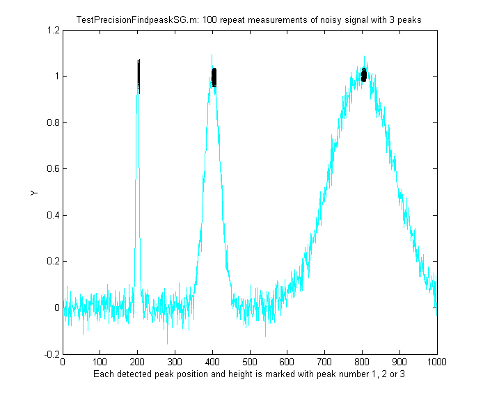 TestPrecisionFindpeaksSG.m
creates a noisy signal with three peaks of widely different
widths, detects and measures the peak positions, heights and
widths of each peak using findpeaksSG, then prints out the percent
relative standard deviations of parameters of the three peaks in
100 measurements with independent random noise. With 3-segment
peak detection parameters, findpeaksSG reliably detects and
accurately measures all three peaks. In contrast, findpeaksG,
tuned to the middle peak (using line 26 instead of line 25),
measures the first and last peaks poorly, because the peak
detection parameters are far from optimum for those peak widths.
You can also see that the precision of peak height
measurements gets progressively better (smaller relative
standard deviation) the larger the peak widths, simply
because there are more data points in wider peaks. (You
can change any of the variables in lines 10-18).
TestPrecisionFindpeaksSG.m
creates a noisy signal with three peaks of widely different
widths, detects and measures the peak positions, heights and
widths of each peak using findpeaksSG, then prints out the percent
relative standard deviations of parameters of the three peaks in
100 measurements with independent random noise. With 3-segment
peak detection parameters, findpeaksSG reliably detects and
accurately measures all three peaks. In contrast, findpeaksG,
tuned to the middle peak (using line 26 instead of line 25),
measures the first and last peaks poorly, because the peak
detection parameters are far from optimum for those peak widths.
You can also see that the precision of peak height
measurements gets progressively better (smaller relative
standard deviation) the larger the peak widths, simply
because there are more data points in wider peaks. (You
can change any of the variables in lines 10-18). a signal (shown on the right)
that might be interpreted as either one peak at x=3 on a
curved baseline or as two peaks at x=.5
and x=3, depending on
context. The peak finding algorithms described here have input
arguments that allow some latitude for adjustment. In this
example script, the "SlopeThreshold" argument is adjusted to
detect just one or both of those peaks.
a signal (shown on the right)
that might be interpreted as either one peak at x=3 on a
curved baseline or as two peaks at x=.5
and x=3, depending on
context. The peak finding algorithms described here have input
arguments that allow some latitude for adjustment. In this
example script, the "SlopeThreshold" argument is adjusted to
detect just one or both of those peaks.  individually by simple keypresses and displays the
results graphically and instantly. The script
FindpeaksComparison
shows how findpeakG compares to
the other peak detection functions
when applied
to a
computer-generated signal with
multiple peaks with variable types
and amounts of baseline and random
noise. By itself, autofindpeaks.m,
findpeaksG and findpeaksL do not
correct for a non-zero
baseline; if your
peaks are superimposed on a
baseline, you should subtract the
baseline first or use
the
other peak detection functions
that do correct for the baseline.
individually by simple keypresses and displays the
results graphically and instantly. The script
FindpeaksComparison
shows how findpeakG compares to
the other peak detection functions
when applied
to a
computer-generated signal with
multiple peaks with variable types
and amounts of baseline and random
noise. By itself, autofindpeaks.m,
findpeaksG and findpeaksL do not
correct for a non-zero
baseline; if your
peaks are superimposed on a
baseline, you should subtract the
baseline first or use
the
other peak detection functions
that do correct for the baseline.
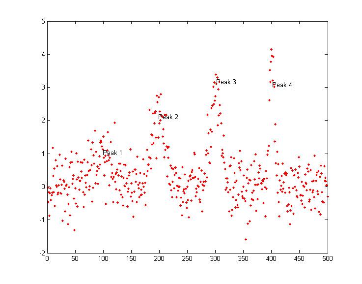 a direct comparison of the accuracy of findpeaksG vs
peakfit, run the demonstration script peakfitVSfindpeaks.m.
This script generates four very noisy peaks of different
heights and widths, then measures them in two different
ways: first with findpeaksG.m (figure on the left) and
then with peakfit.m, and
compares the results. The peaks detected by findpeaksG are
labeled "Peak 1", "Peak 2", etc. If you run this script
several times, it will generate the same peaks but with independent
samples of the random noise each time. You'll find
that both methods work well most of the time, with peakfit
giving smaller errors in most cases (because it uses all
the points in each peak, not just the top part), but
occasionally findpeaksG will miss the first (lowest) peak
and rarely it will detect an 5th peak that is not really
there. On the other hand, peakfit.m is constrained to fit
4 and only 4 peaks each time.
a direct comparison of the accuracy of findpeaksG vs
peakfit, run the demonstration script peakfitVSfindpeaks.m.
This script generates four very noisy peaks of different
heights and widths, then measures them in two different
ways: first with findpeaksG.m (figure on the left) and
then with peakfit.m, and
compares the results. The peaks detected by findpeaksG are
labeled "Peak 1", "Peak 2", etc. If you run this script
several times, it will generate the same peaks but with independent
samples of the random noise each time. You'll find
that both methods work well most of the time, with peakfit
giving smaller errors in most cases (because it uses all
the points in each peak, not just the top part), but
occasionally findpeaksG will miss the first (lowest) peak
and rarely it will detect an 5th peak that is not really
there. On the other hand, peakfit.m is constrained to fit
4 and only 4 peaks each time. is a segmented
variant of findpeaksb.m. It has
the same syntax as findpeaksb.m,
except that the input arguments
SlopeThreshold, AmpThreshold,
smoothwidth, peakgroup, window, width,
PeakShape, extra, NumTrials, autozero,
and fixedparameters, can all
optionally be scalars or vectors with
one entry for each segment, in the
same manner as findpeaksSG.m.
Returns a matrix P listing the peak
number, position, height, width, area,
percent fitting error and "R2" of each
detected peak. In the example on the
right, the two peaks have the same
height above baseline (1.00) but
different shapes (the first Lorentzian
and the second Gaussian), very
different widths, and different
baselines. So, using findpeaksG or
findpeaksL or findpeaksb, it would be
impossible to find one set of input
arguments that would be optimum for
both peaks. But, using
findpeaksSb.m, different settings can
apply to different regions of the
signal. In this simple example, there
are only two segments,
defined by SlopeThreshold with 2
different values, and the other input
arguments are either the same or are
different in those two segments. The
result is that the peak height of the
both peaks is measured accurately.
is a segmented
variant of findpeaksb.m. It has
the same syntax as findpeaksb.m,
except that the input arguments
SlopeThreshold, AmpThreshold,
smoothwidth, peakgroup, window, width,
PeakShape, extra, NumTrials, autozero,
and fixedparameters, can all
optionally be scalars or vectors with
one entry for each segment, in the
same manner as findpeaksSG.m.
Returns a matrix P listing the peak
number, position, height, width, area,
percent fitting error and "R2" of each
detected peak. In the example on the
right, the two peaks have the same
height above baseline (1.00) but
different shapes (the first Lorentzian
and the second Gaussian), very
different widths, and different
baselines. So, using findpeaksG or
findpeaksL or findpeaksb, it would be
impossible to find one set of input
arguments that would be optimum for
both peaks. But, using
findpeaksSb.m, different settings can
apply to different regions of the
signal. In this simple example, there
are only two segments,
defined by SlopeThreshold with 2
different values, and the other input
arguments are either the same or are
different in those two segments. The
result is that the peak height of the
both peaks is measured accurately.  findpeaksb3.m
is a more ambitious variant of findpeaksb.m that fits each
detected peak along with the previous and following peaks
found by findpeaksG.m, so as to deal better with overlap of
the adjacent overlapping peaks. The syntax is function FPB=findpeaksb3(x,y,
SlopeThreshold, AmpThreshold, smoothwidth, peakgroup,
smoothtype, PeakShape, extra, NumTrials, AUTOZERO, ShowPlots).
The demonstration script DemoFindPeaksb3.m shows
how findpeaksb3 works with irregular clusters of
overlapping Lorentzian peaks, as in the example on
the left (type "help findpeaksb3") for more.
The
demonstration
script FindpeaksComparison
shows how findpeaksb3 compares to the
other peak detection functions when
applied to signals with multiple peaks
and variable types and amounts of
baseline and random noise.
findpeaksb3.m
is a more ambitious variant of findpeaksb.m that fits each
detected peak along with the previous and following peaks
found by findpeaksG.m, so as to deal better with overlap of
the adjacent overlapping peaks. The syntax is function FPB=findpeaksb3(x,y,
SlopeThreshold, AmpThreshold, smoothwidth, peakgroup,
smoothtype, PeakShape, extra, NumTrials, AUTOZERO, ShowPlots).
The demonstration script DemoFindPeaksb3.m shows
how findpeaksb3 works with irregular clusters of
overlapping Lorentzian peaks, as in the example on
the left (type "help findpeaksb3") for more.
The
demonstration
script FindpeaksComparison
shows how findpeaksb3 compares to the
other peak detection functions when
applied to signals with multiple peaks
and variable types and amounts of
baseline and random noise.  The first
seven input arguments are exactly the same as for the findpeaksG.m
function; if you have been using findpeaksG
or iPeak to find and measure peaks in your
signals, you can use those same input argument values for
findpeaksfit.m. The remaining six input arguments of
findpeaksfit.m are for the peakfit
function; if you have been using peakfit.m or ipf.m
to fit the peaks in your signals, then you can use those same
input argument values for findpeaksfit.m.
The
demonstration script findpeaksfitdemo.m,
shows findpeaksfit automatically finding and fitting the peaks in
a set of 150 signals, each of which may have 1 to 3 noisy
Lorentzian peaks in variable locations, artificially slowed
down with the "pause" function so you can see it better.
Requires the findpeaksfit.m and lorentzian.m functions installed. This
script was used to generate the GIF animation shown on the left.
Type "help findpeaksfit" for more information.
The first
seven input arguments are exactly the same as for the findpeaksG.m
function; if you have been using findpeaksG
or iPeak to find and measure peaks in your
signals, you can use those same input argument values for
findpeaksfit.m. The remaining six input arguments of
findpeaksfit.m are for the peakfit
function; if you have been using peakfit.m or ipf.m
to fit the peaks in your signals, then you can use those same
input argument values for findpeaksfit.m.
The
demonstration script findpeaksfitdemo.m,
shows findpeaksfit automatically finding and fitting the peaks in
a set of 150 signals, each of which may have 1 to 3 noisy
Lorentzian peaks in variable locations, artificially slowed
down with the "pause" function so you can see it better.
Requires the findpeaksfit.m and lorentzian.m functions installed. This
script was used to generate the GIF animation shown on the left.
Type "help findpeaksfit" for more information.  amounts of
baseline and random noise. (Requires those four functions, plus
gaussian.m, lorentzian.m, modelpeaks.m, findpeaksG.m,
findpeaksL.m, pinknoise.m, and propnoise.m, in the Matlab/Octave
path). Results are displayed graphically in figure windows 1, 2, and 3 and printed out in a table of
parameter accuracy and elapsed time for each method, as shown
below. You may change the lines in the script marked
by <<< to modify the number and character and amplitude
of the signal peaks, baseline, and noise. Make the signal
similar to yours to discover which method works best for your type
of signal. The best method depends mainly on the shape and
amplitude of the baseline and on the extent of peak overlap. Type
"help FindpeaksComparison"
for details. (Times updated for Matlab 2020 on
Dell XPS i7
3.5Ghz).
amounts of
baseline and random noise. (Requires those four functions, plus
gaussian.m, lorentzian.m, modelpeaks.m, findpeaksG.m,
findpeaksL.m, pinknoise.m, and propnoise.m, in the Matlab/Octave
path). Results are displayed graphically in figure windows 1, 2, and 3 and printed out in a table of
parameter accuracy and elapsed time for each method, as shown
below. You may change the lines in the script marked
by <<< to modify the number and character and amplitude
of the signal peaks, baseline, and noise. Make the signal
similar to yours to discover which method works best for your type
of signal. The best method depends mainly on the shape and
amplitude of the baseline and on the extent of peak overlap. Type
"help FindpeaksComparison"
for details. (Times updated for Matlab 2020 on
Dell XPS i7
3.5Ghz).
 findpeaksG2d.m
is a variant of findpeaksSG that can be used to locate the
positive peaks and shoulders in a noisy x-y time series
data set. Detects peaks in the negative of the second
derivative of the signal, by looking for downward slopes in
the third derivative that exceed SlopeThreshold. See TestFindpeaksG2d.m.
findpeaksG2d.m
is a variant of findpeaksSG that can be used to locate the
positive peaks and shoulders in a noisy x-y time series
data set. Detects peaks in the negative of the second
derivative of the signal, by looking for downward slopes in
the third derivative that exceed SlopeThreshold. See TestFindpeaksG2d.m.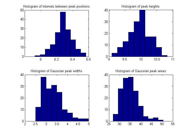
 The problem with this method
is that it requires an analytical peak model, expressed as a
closed-form expression, that can be solved algebraically for
their start and end points. A more versatile method is to fit
a model to the peak data by iterative
curve fitting, and then use the best-fit model to locate
the start and stop points by interpolation. For complex peak
shapes, the model need not be limited to a single peak;
very often complex peak shapes can be modeled as the sum of
simple shapes, such as Gaussians. An example of this method is
demonstrated in the script StartAndEnd.m,
which simulates a noisy, asymmetrical peak and then applies
this method using the downloadable peakfit.m
function. You can select the start/stop cut-off point as a
fraction of the peak height in line 8 and the amount or random
noise in line 7. The default for both values is 0.01 (or 1%),
which means that, at the cut-off points, the signal-to-noise
ratio is very poor. Nevertheless, the start and end points can
be calculated surprisingly precisely, because they are
calculated from the best-fit model (contained in the output
arguments xi and yi of the peakfit function), which averages
out the noise over the entire signal (the more data points the
better). The animation on the left shows the method in
operation for 50 repeat measurements with different random
noise samples, first with 1% noise and then with 10% noise.
Despite the poor signal-to-noise ratio at the cut-off points,
the relative standard deviation of the measured start and end
times (marked by the vertical lines) is only about 0.2%. (Even
when the noise is increased 10-fold to 0.1 in line 7, the
results are still surprisingly good).
The problem with this method
is that it requires an analytical peak model, expressed as a
closed-form expression, that can be solved algebraically for
their start and end points. A more versatile method is to fit
a model to the peak data by iterative
curve fitting, and then use the best-fit model to locate
the start and stop points by interpolation. For complex peak
shapes, the model need not be limited to a single peak;
very often complex peak shapes can be modeled as the sum of
simple shapes, such as Gaussians. An example of this method is
demonstrated in the script StartAndEnd.m,
which simulates a noisy, asymmetrical peak and then applies
this method using the downloadable peakfit.m
function. You can select the start/stop cut-off point as a
fraction of the peak height in line 8 and the amount or random
noise in line 7. The default for both values is 0.01 (or 1%),
which means that, at the cut-off points, the signal-to-noise
ratio is very poor. Nevertheless, the start and end points can
be calculated surprisingly precisely, because they are
calculated from the best-fit model (contained in the output
arguments xi and yi of the peakfit function), which averages
out the noise over the entire signal (the more data points the
better). The animation on the left shows the method in
operation for 50 repeat measurements with different random
noise samples, first with 1% noise and then with 10% noise.
Despite the poor signal-to-noise ratio at the cut-off points,
the relative standard deviation of the measured start and end
times (marked by the vertical lines) is only about 0.2%. (Even
when the noise is increased 10-fold to 0.1 in line 7, the
results are still surprisingly good).  and
findpeaksTplot.m are
variants of findpeaksG that measure the peak parameters by automatically
constructing a triangle around each peak with its sides
tangent to the sides of the peak, as shown on the right (script that generated this graphic).
This method mimics the geometric construction method that was
formerly used to measure peak parameters manually before the
age of computers. Peak height is taken as the apex of the
triangle, which is slightly higher than the peak of the
underlying curve. The performance of this method is poor when
the signals are very noisy or if the peaks overlap, but in a
few circumstances the triangle construction
method might be more accurate for the measurement of
peak area than the Gaussian method, especially if the peaks
are asymmetric or of uncertain shape (see the
demo function triangulationdemo.m
for some examples: click for
graphic).
and
findpeaksTplot.m are
variants of findpeaksG that measure the peak parameters by automatically
constructing a triangle around each peak with its sides
tangent to the sides of the peak, as shown on the right (script that generated this graphic).
This method mimics the geometric construction method that was
formerly used to measure peak parameters manually before the
age of computers. Peak height is taken as the apex of the
triangle, which is slightly higher than the peak of the
underlying curve. The performance of this method is poor when
the signals are very noisy or if the peaks overlap, but in a
few circumstances the triangle construction
method might be more accurate for the measurement of
peak area than the Gaussian method, especially if the peaks
are asymmetric or of uncertain shape (see the
demo function triangulationdemo.m
for some examples: click for
graphic).  findsteps.m, syntax:
P=findpulses(x, y, SlopeThreshold, AmpThreshold, SmoothWidth,
peakgroup), locates positive transient steps in noisy x-y time
series data, by computing the first derivative of y that exceed
SlopeThreshold, computes the step height as the difference between
the maximum and minimum y values over a number of data point equal
to "Peakgroup". Returns list (P) with step number, x position, y
position, and the step height of each step detected;
"SlopeThreshold" and "AmpThreshold" control step sensitivity;
higher values will neglect smaller features.
Increasing "SmoothWidth" reduces small sharp false steps caused by
random noise or by "glitches" in the data acquisition. See findsteps.png for a real example. And findstepsplot.m plots the signal and
numbers the peaks.
findsteps.m, syntax:
P=findpulses(x, y, SlopeThreshold, AmpThreshold, SmoothWidth,
peakgroup), locates positive transient steps in noisy x-y time
series data, by computing the first derivative of y that exceed
SlopeThreshold, computes the step height as the difference between
the maximum and minimum y values over a number of data point equal
to "Peakgroup". Returns list (P) with step number, x position, y
position, and the step height of each step detected;
"SlopeThreshold" and "AmpThreshold" control step sensitivity;
higher values will neglect smaller features.
Increasing "SmoothWidth" reduces small sharp false steps caused by
random noise or by "glitches" in the data acquisition. See findsteps.png for a real example. And findstepsplot.m plots the signal and
numbers the peaks. Rectangular
pulses (square waves) require a different approach, based
on amplitude discrimination rather than differentiation. The
function "findsquarepulse.m"
(syntax S=findsquarepulse(t,y,threshold) locates the
rectangular pulses in the signal t,y that exceed a y-value of
"threshold" and determines their start time, average height
(relative to the baseline) and width. DemoFindsquare.m creates a test signal
(with a true height of 2636 and a height of 750) and calls findsquarepulse.m
to demonstrate. If the signal is very noisy, some preliminary
rectangular smoothing (e.g. using fastsmooth.m) before calling
findsquarepulse.m may be helpful to eliminate false peaks.
Rectangular
pulses (square waves) require a different approach, based
on amplitude discrimination rather than differentiation. The
function "findsquarepulse.m"
(syntax S=findsquarepulse(t,y,threshold) locates the
rectangular pulses in the signal t,y that exceed a y-value of
"threshold" and determines their start time, average height
(relative to the baseline) and width. DemoFindsquare.m creates a test signal
(with a true height of 2636 and a height of 750) and calls findsquarepulse.m
to demonstrate. If the signal is very noisy, some preliminary
rectangular smoothing (e.g. using fastsmooth.m) before calling
findsquarepulse.m may be helpful to eliminate false peaks.


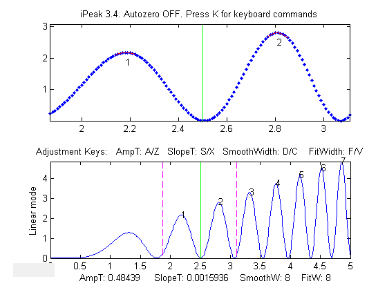

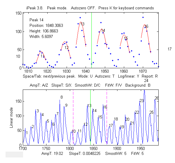

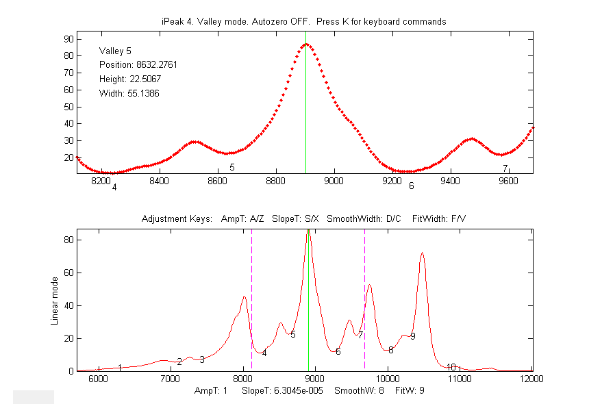
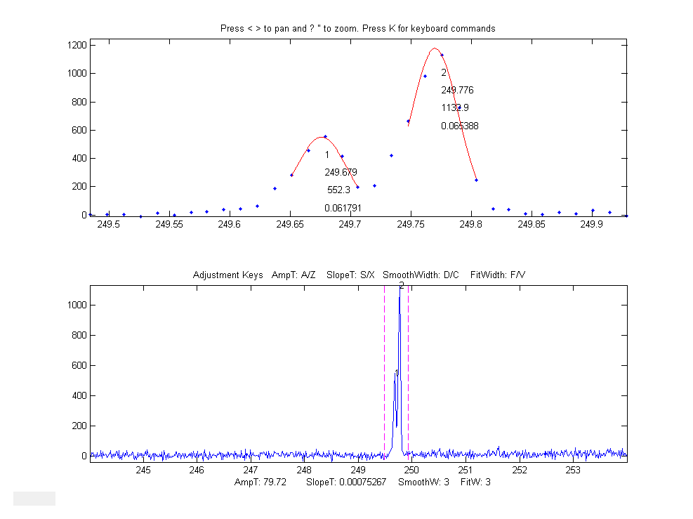

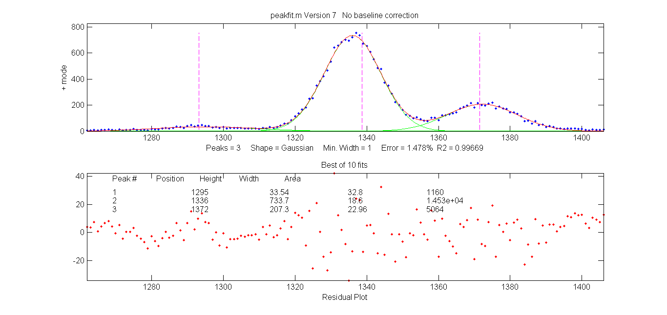
 This example generates four Gaussian
peaks, all with the exact same peak height (1.00) and area
(1.773). The first peak (at x=4) is isolated, the second peak
(x=9) is slightly overlapped with the third one, and the last two
peaks (at x= 13 and 15) are strongly overlapped.
This example generates four Gaussian
peaks, all with the exact same peak height (1.00) and area
(1.773). The first peak (at x=4) is isolated, the second peak
(x=9) is slightly overlapped with the third one, and the last two
peaks (at x= 13 and 15) are strongly overlapped. itself, iPeak does a fairly good
just of measuring peaks positions and heights by fitting just
the top part of the peaks, because the peaks are Gaussian, but
the areas and
widths of the last two
peaks (which should be 1.665 like the others) are quite a bit too large because of the overlap:
itself, iPeak does a fairly good
just of measuring peaks positions and heights by fitting just
the top part of the peaks, because the peaks are Gaussian, but
the areas and
widths of the last two
peaks (which should be 1.665 like the others) are quite a bit too large because of the overlap: 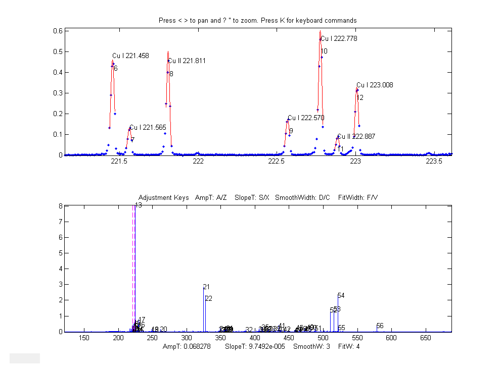
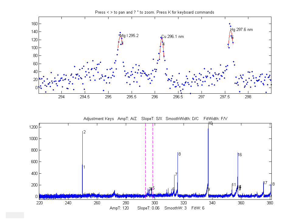

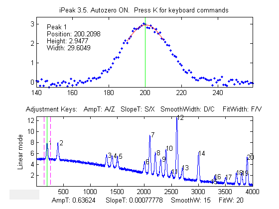
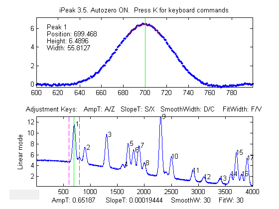
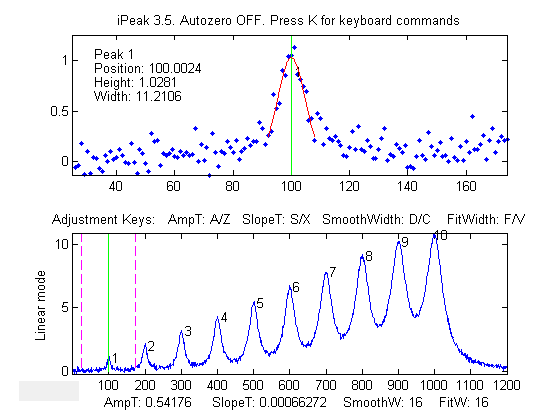
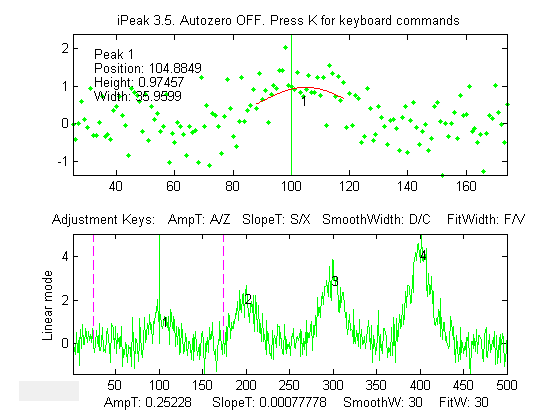

