[Smoothing Algorithms] [Savitzky-Golay] [[Noise Reduction] [End Effects] [Examples] [The problem with smoothing] [Optimization] [When should you smooth a signal?] [When should you NOT smooth a signal?] [Dealing with spikes] [Video Demonstration] [Spreadsheets] [Matlab/Octave] [Live Script] [Interactive tools] [Have a question? Email me]
In many experiments in science, the true signal amplitudes (y-axis
values) change rather smoothly as a function of the x-axis values, whereas many kinds of noise are seen as
rapid, random changes in amplitude from point to point within
the signal. In the latter situation it may be useful in some
cases to attempt to reduce the noise by a process called smoothing. In smoothing,
the data points of a signal are modified so that individual
points that are higher than the immediately adjacent points (presumably
because of noise) are reduced, and points that are lower than the adjacent
points are increased. This naturally leads to a smoother signal
(and a slower step response to signal changes). As long as the
true underlying signal is actually smooth, then the true signal
will not be much distorted by smoothing, but the high frequency
noise will be reduced. In terms of the frequency components
of a signal, a smoothing operation acts as a low-pass
filter, reducing the high-frequency components and passing
the low-frequency components with little change. If the signal
and the noise is measured over all frequencies, then the signal-to-noise ratio will
be improved by smoothing, by an amount that depends on the frequency distribution of the noise.
many experiments in science, the true signal amplitudes (y-axis
values) change rather smoothly as a function of the x-axis values, whereas many kinds of noise are seen as
rapid, random changes in amplitude from point to point within
the signal. In the latter situation it may be useful in some
cases to attempt to reduce the noise by a process called smoothing. In smoothing,
the data points of a signal are modified so that individual
points that are higher than the immediately adjacent points (presumably
because of noise) are reduced, and points that are lower than the adjacent
points are increased. This naturally leads to a smoother signal
(and a slower step response to signal changes). As long as the
true underlying signal is actually smooth, then the true signal
will not be much distorted by smoothing, but the high frequency
noise will be reduced. In terms of the frequency components
of a signal, a smoothing operation acts as a low-pass
filter, reducing the high-frequency components and passing
the low-frequency components with little change. If the signal
and the noise is measured over all frequencies, then the signal-to-noise ratio will
be improved by smoothing, by an amount that depends on the frequency distribution of the noise.
Smoothing algorithms. Most smoothing algorithms are based on the "shift and multiply" technique, in which a group of adjacent points in the original data are multiplied point-by-point by a set of numbers (coefficients) that defines the smooth shape, the products are added up and divided by the sum of the coefficients, which becomes one point of smoothed data, then the set of coefficients is shifted one point down the original data and the process is repeated. The simplest smoothing algorithm is the rectangular boxcar or unweighted sliding-average smooth; it simply replaces each point in the signal with the average of m adjacent points, where m is a positive integer called the smooth width. For example, for a 3-point smooth (m = 3):
![]()
for j = 2 to n-1, where Sj the jth point in the smoothed signal, Yj the jth point in the original signal, and n is the total number of points in the signal. Similar smooth operations can be constructed for any desired smooth width, m. Usually m is an odd number. If the noise in the data is "white noise" (that is, evenly distributed over all frequencies) and its standard deviation is D, then the standard deviation of the noise remaining in the signal after the first pass of an unweighted sliding-average smooth will be approximately D over the square root of m (D/sqrt(m)), where m is the smooth width. Despite its simplicity, this smooth is actually optimum for the common problem of reducing white noise while keeping the sharpest step response. The response to a step change is in fact linear, so this filter has the advantage of responding completely with no residual effect within its response time, which is equal to the smooth width divided by the sampling rate. Smoothing can be performed either during data acquisition, by programming the digitizer to measure and average multiple readings and save only the average, or after data acquisition ("post-run"), by storing all the acquired data in memory and smoothing the stored data. The latter requires more memory but is more flexible.
The triangular smooth is like the rectangular smooth, above, except that it implements a weighted smoothing function. For a 5-point smooth (m = 5):
![]()
for j = 3 to n-2, and similarly for other smooth widths
(see the spreadsheet UnitGainSmooths.xls).
In
both of these cases, the integer in the denominator is the sum of the coefficients in
the numerator, which results in a "unit-gain" smooth that has no
effect on the signal where it is a straight line and which
preserves the area under peaks.
It is often useful to apply a smoothing operation more than
once, that is, to smooth an already smoothed signal, in order to
build longer and more complicated smooths. For example, the
5-point triangular smooth above is equivalent to two passes of a
3-point rectangular smooth. Three passes of a 3-point rectangular smooth result in a
7-point "pseudo-Gaussian" or haystack smooth, for which the coefficients are in the ratio
1:3:6:7:6:3:1. The general rule is that n passes of a w-width smooth results in a combined smooth width of n*w-n+1.
For example, 3 passes of a 17-point smooth results in a 49-point
smooth. These multi-pass smooths are more effective at reducing
high-frequency noise in the signal than a rectangular smooth,
but they exhibit slower step response.
In all these smooths, the width of the smooth m is chosen to be an odd
integer, so that the smooth coefficients are symmetrically
balanced around the central point, which is important because it
preserves the x-axis position of peaks and other features in the
smoothed signal. (This is especially critical for analytical and
spectroscopic applications because the peak positions are often
important measurement objectives).
Note that we are assuming here that the x-axis intervals of the
signal is uniform, that is, that the difference between the
x-axis values of adjacent points is the same throughout the
signal. This is also assumed in many of the other
signal-processing techniques described in this essay, and it is
a very common (but not necessary) characteristic of signals that
are acquired by automated and computerized equipment.
The Savitzky-Golay
smooth is a very widely-used smoothing algorithm that is based
on the least-squares fitting of polynomials to segments of the
data. The algorithm is discussed in http://www.wire.tu-bs.de/OLDWEB/mameyer/cmr/savgol.pdf.
Compared to the sliding-average smooths of the same width, the
Savitzky-Golay smooth is less effective at reducing noise, but more
effective at retaining the shape of the original signal.
It is capable of differentiation
as well as smoothing. The algorithm is more complex and
the computational times may be greater than the smooth types
discussed above, but with modern computers the difference is not
significant. Code
in
various languages is widely available online. See SmoothingComparison.html.
The shape of any smoothing algorithm can be determined by
applying that smooth to a signal
consisting of all zeros except for one point, called a delta
function or impulse,
as demonstrated by the simple Matlab/Octave script DeltaTest.m.
The result is called the
impulse response function (Graphic).
Noise reduction.
Smoothing usually reduces the noise in a signal. If the noise is
"white" (that is, evenly distributed over all frequencies) and
its standard deviation is D, then the standard deviation of the noise remaining in
the signal after one pass of a rectangular smooth will be
approximately D/sqrt(m), where m is the smooth width. If a triangular smooth is used
instead, the noise will be slightly less, about D*0.8/sqrt(m). Smoothing operations can be applied more than once:
that is, a previously-smoothed signal can be smoothed again. In
some cases this can be useful if there is a great deal of
high-frequency noise in the signal. However, the noise
reduction for white noise is less in each successive
smooth. For example, three passes of a rectangular smooth reduces white noise by a
factor of approximately D*0.7/sqrt(m), only a slight improvement over two passes. For
a spreadsheet demonstration, see VariableSmoothNoiseReduction.xlsx.
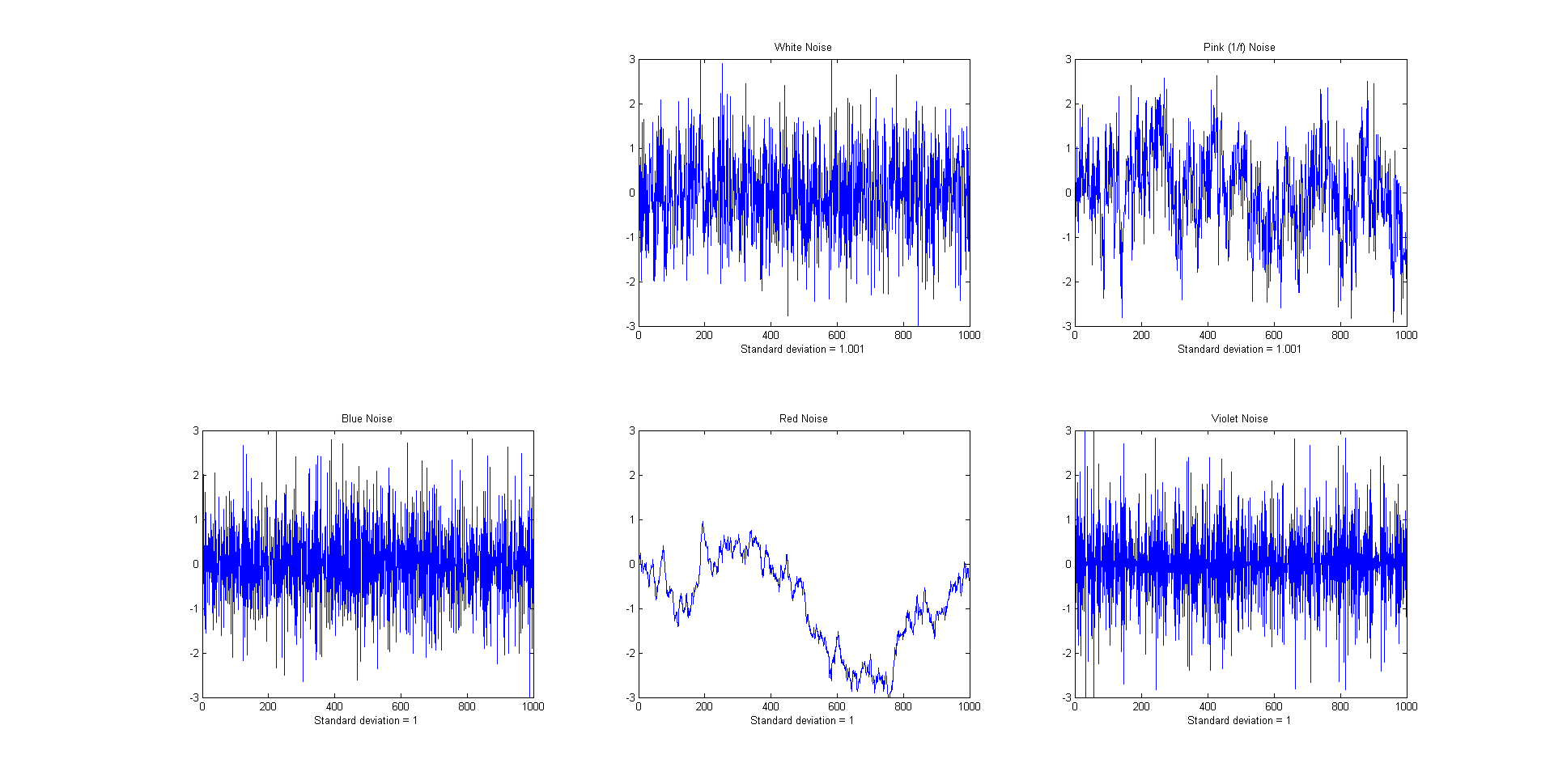
 The frequency distribution of noise,
designated by noise
color, substantially effects the ability of smoothing to
reduce noise. The Matlab/Octave function "NoiseColorTest.m" compares the
effect of a 20-point boxcar (unweighted sliding average) smooth
on the standard deviation of white, pink, red, and blue noise,
all of which have an original
unsmoothed standard deviation of 1.0. Because smoothing is
a low-pass filter process, it effects low frequency (pink and
red) noise less, and effects high-frequency (blue and violet)
noise more, than it does white noise.
The frequency distribution of noise,
designated by noise
color, substantially effects the ability of smoothing to
reduce noise. The Matlab/Octave function "NoiseColorTest.m" compares the
effect of a 20-point boxcar (unweighted sliding average) smooth
on the standard deviation of white, pink, red, and blue noise,
all of which have an original
unsmoothed standard deviation of 1.0. Because smoothing is
a low-pass filter process, it effects low frequency (pink and
red) noise less, and effects high-frequency (blue and violet)
noise more, than it does white noise.
|
Original unsmoothed noise |
1 |
|
Smoothed white noise |
0.1 |
|
Smoothed pink noise |
0.55 |
|
Smoothed blue noise |
0.01 |
|
Smoothed red (random walk) noise |
0.98 |
Note that the computation of standard
deviation is independent of the order of the data and thus of
its frequency distribution; sorting a set of data does not
change its standard deviation. The standard deviation of a
sine wave is independent of its frequency. Smoothing, however,
changes both the frequency distribution and standard deviation
of a data set.
End effects and the lost points problem. In the equations above, the 3-point rectangular smooth is defined only for j = 2 to n-1. There is not enough data in the signal to define a complete 3-point smooth for the first point in the signal (j = 1) or for the last point (j = n) , because there are no data points before the first point or after the last point. (Similarly, a 5-point smooth is defined only for j = 3 to n-2, and therefore a smooth can not be calculated for the first two points or for the last two points). In general, for an m-width smooth, there will be (m-1)/2 points at the beginning of the signal and (m-1)/2 points at the end of the signal for which a complete m-width smooth can not be calculated the usual way. What to do? There are two approaches. One is to accept the loss of points and trim off those points or replace them with zeros in the smooth signal. (That's the approach taken in most of the figures in this paper). The other approach is to use progressively smaller smooths at the ends of the signal, for example to use 2, 3, 5, 7... point smooths for signal points 1, 2, 3,and 4..., and for points n, n-1, n-2, n-3..., respectively. The later approach may be preferable if the edges of the signal contain critical information, but it increases execution time. The Matlb/Octave fastsmooth function discussed below can utilize either of these two methods.
Examples of smoothing. A simple example of smoothing is shown in Figure 4. The left half of this signal is a noisy peak. The right half is the same peak after undergoing a triangular smoothing algorithm. The noise is greatly reduced while the peak itself is hardly changed. The reduced noise allows the signal characteristics (peak position, height, width, area, etc.) to be measured more accurately by visual inspection.

Figure 4. The left half of this signal is a noisy peak. The right half is the same peak after undergoing a smoothing algorithm. The noise is greatly reduced while the peak itself is hardly changed, making it easier to measure the peak position, height, and width directly by graphical or visual estimation (but it does not improve measurements made by least-squares methods; see below).
The larger the smooth width, the greater the noise reduction, but also the greater the possibility that the signal will be distorted by the smoothing operation. The optimum choice of smooth width depends upon the width and shape of the signal and the digitization interval. For peak-type signals, the critical factor is the smooth ratio, the ratio between the smooth width m and the number of points in the half-width of the peak. In general, increasing the smoothing ratio improves the signal-to-noise ratio but causes a reduction in amplitude and in increase in the bandwidth of the peak. Be aware that the smooth width can be expressed in two different ways: (a) as the number of data points or (b) as the x-axis interval (for spectroscopic data usually in nm or in frequency units). The two are simply related: the number of data points is simply the x-axis interval times the increment between adjacent x-axis values. The smooth ratio is the same in either case.


The figures above show examples of the effect of three different smooth widths on noisy Gaussian-shaped peaks. In the figure on the left, the peak has a true height of 2.0 and there are 80 points in the half-width of the peak. The red line is the original unsmoothed peak. The three superimposed green lines are the results of smoothing this peak with a triangular smooth of width (from top to bottom) 7, 25, and 51 points. Because the peak width is 80 points, the smooth ratios of these three smooths are 7/80 = 0.09, 25/80 = 0.31, and 51/80 = 0.64, respectively. As the smooth width increases, the noise is progressively reduced but the peak height also is reduced slightly. For the largest smooth, the peak width is noticeably increased. In the figure on the right, the original peak (in red) has a true height of 1.0 and a half-width of 33 points. (It is also less noisy than the example on the left.) The three superimposed green lines are the results of the same three triangular smooths of width 7, 25, and 51 points. But because the peak width in this case is only 33 points, the smooth ratios of these three smooths are larger - 0.21, 0.76, and 1.55, respectively. You can see that the peak distortion effect (reduction of peak height and increase in peak width) is greater for the narrower peak because the smooth ratios are higher. Smooth ratios of greater than 1.0 are seldom used because of excessive peak distortion. Note that even in the worst case, the peak positions are not effected (assuming that the original peaks were symmetrical and not overlapped by other peaks). If retaining the shape of the peak is more important than optimizing the signal-to-noise ratio, the Savitzky-Golay has the advantage over sliding-average smooths. In all cases, the total area under the peak remains unchanged. If the peak widths vary substantially, an adaptive smooth, which allows the smooth width to vary across the signal, may be used.
The problem with smoothing is that it is often less beneficial than you might think. It's important to point out that smoothing results such as illustrated in the figure above may be deceptively impressive because they employ a single sample of a noisy signal that is smoothed to different degrees. This causes the viewer to underestimate the contribution of low-frequency noise, which is hard to estimate visually because there are so few low-frequency cycles in the signal record. This problem can visualized by recording a number of independent samples of a noisy signal consisting of a single peak, as illustrated in the two figures below. These figures show ten superimposed plots with the same peak but with independent white noise, each plotted with a different line color, unsmoothed on the left and smoothed on the right. Clearly, the noise reduction is substantial, but close inspection of the smoothed signals on the right clearly shows the variation in peak position, height, and width between the 10 samples caused by the low frequency noise remaining in the smoothed signals. Without the noise, each peak would have a peak height of 2, peak center at 500, and width of 150. Just because a signal looks smooth does not mean there is no noise. Low-frequency noise remaining in the signals after smoothing will still interfere with precise measurement of peak position, height, and width.
|
|
|
|
x=1:1000; |
x=1:1000; |
(The generating scripts below each figure require that the functions gaussian.m, whitenoise.m, and fastsmooth.m be downloaded from http://tinyurl.com/cey8rwh.)
It should be clear that smoothing can seldom completely eliminate noise, because most noise is spread out over a range of frequencies, and smoothing simply reduces the noise in part of its frequency range. Only for some very specific types of noise (e.g. discrete frequency sine-wave noise or single-point spikes) is there hope of anything close to complete noise elimination. Smoothing does make the signal smoother and it does reduce the standard deviation of the noise, but whether or not that makes for a better measurement or not depends on the situation. And don't assume that just because a little smoothing is good that more will necessarily be better. Smoothing is like alcohol; sometimes you really need it - but you should never overdo it.
The figure on the right below is another example
signal that illustrates some of these principles. The signal
consists of two Gaussian peaks, one located at x=50 and the
second at x=150. Both peaks have a peak height of 1.0 and a peak
half-width of 10, and the same normally-distributed random white
noise with a standard deviation of 0.1 has been added to the
entire signal. The x-axis sampling interval, however, is
different for the two peaks; it's 0.1 for the first peak (from
x=0 to 100) and 1.0 for the second peak (from x=100 to
200). This means that the first peak is 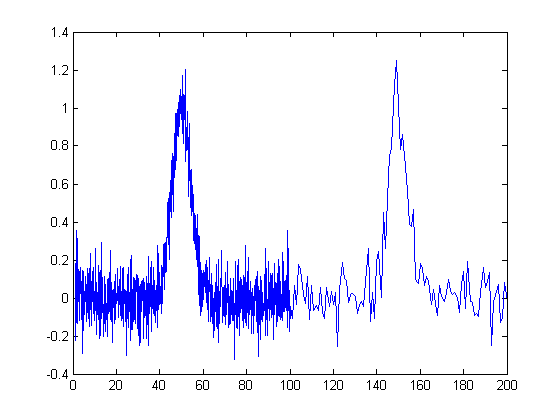 characterized
by
ten times more points that the second peak. It may look like the first peak
is noisier than the second, but that's just an illusion; the
signal-to-noise ratio for both peaks is 10. The second peak
looks less noisy only because there are fewer noise samples
there and we tend to underestimate the dispersion of small
samples. The result of this is that when the signal is smoothed,
the second peak is much more likely to be distorted by
the smooth (it becomes shorter and wider) than the first peak.
The first peak can tolerate a much wider smooth width, resulting
in a greater degree of noise reduction. (Similarly, if both
peaks are measured with the least-squares
curve fitting method to be covered later, the fit of the first peak is more
stable with the noise and the measured parameters of that
peak will be about 3 times more
accurate than the second peak,
because there are 10 times more data points in that peak, and
the measurement precision improves roughly with the square root
of the number of data points if the noise is white). You
can download this data file, "udx", in TXT
format or in Matlab MAT format.
characterized
by
ten times more points that the second peak. It may look like the first peak
is noisier than the second, but that's just an illusion; the
signal-to-noise ratio for both peaks is 10. The second peak
looks less noisy only because there are fewer noise samples
there and we tend to underestimate the dispersion of small
samples. The result of this is that when the signal is smoothed,
the second peak is much more likely to be distorted by
the smooth (it becomes shorter and wider) than the first peak.
The first peak can tolerate a much wider smooth width, resulting
in a greater degree of noise reduction. (Similarly, if both
peaks are measured with the least-squares
curve fitting method to be covered later, the fit of the first peak is more
stable with the noise and the measured parameters of that
peak will be about 3 times more
accurate than the second peak,
because there are 10 times more data points in that peak, and
the measurement precision improves roughly with the square root
of the number of data points if the noise is white). You
can download this data file, "udx", in TXT
format or in Matlab MAT format.
Optimization of smoothing. As smooth width increases, the smoothing ratio increases, noise is reduced quickly at first, then more slowly, and the peak height is also reduced, slowly at first, then more quickly. The noise reduction depends on the smooth width, the smooth type (e.g. rectangular, triangular, etc), and the noise color, but the peak height reduction also depends on the peak width. The result is that the signal-to-noise (defined as the ratio of the peak height of the standard deviation of the noise) increases quickly at first, then reaches a maximum. This is illustrated in the animation at the top of this page for a Gaussian peak with white noise (produced by this Matlab/Octave script). The maximum improvement in the signal-to-noise ratio depends on the number of points in the peak: the more points in the peak, the greater smooth widths can be employed and the greater the noise reduction. This figure also illustrates that most of the noise reduction is due to high frequency components of the noise, whereas much of the low frequency noise remains in the signal even as it is smoothed.
Which is the best smooth ratio? It depends
on the purpose of the peak measurement. If the ultimate
objective of the measurement is to measure the peak height or
width, then smooth ratios below 0.2 should be used and the Savitzky-Golay
smooth is preferred. But if the objective of the measurement is
to measure the peak position (x-axis value of the peak), larger
smooth ratios can be employed if desired, because smoothing has
little effect on the peak position (unless peak is asymmetrical
or the increase in peak width is so much that it causes adjacent
peaks to overlap). If the peak is actually formed of two
underlying peaks that overlap so much that they appear to be one
peak, then curve
fitting is the only way to measure the parameters of the
underlying peaks. Unfortunately, the optimum signal-to-noise
ratio corresponds to a smooth ratio that significantly distorts
the peak, which is why curve fitting the unsmoothed data is
often the preferred method for measuring peaks position, height,
and width. Peak area is not changed by smoothing,
unless it changes your estimate of the beginning and the ending
of the peak.
In quantitative chemical analysis applications based on calibration by standard samples, the peak height reduction caused by smoothing is not so important. If the same signal processing operations are applied to the samples and to the standards, the peak height reduction of the standard signals will be exactly the same as that of the sample signals and the effect will cancel out exactly. In such cases smooth widths from 0.5 to 1.0 can be used if necessary to further improve the signal-to-noise ratio, as shown in the figure on the left (for a simple sliding-average rectangular smooth). In practical analytical chemistry, absolute peak height measurements are seldom required; calibration against standard solutions is the rule. (Remember: the objective of quantitative analysis is not to measure a signal but rather to measure the concentration of the unknown.) It is very important, however, to apply exactly the same signal processing steps to the standard signals as to the sample signals, otherwise a large systematic error will result.
For a more detailed comparison of all four smoothing types considered above, see SmoothingComparison.html.
When should you smooth a signal? There are four reasons to smooth a signal:
(a) for cosmetic reasons, to prepare a nicer-looking or more dramatic graphic of a signal for visual inspection or publications, especially in order to emphasize long-term behavior over short-term, or
(b) If the signal contains mostly high-frequency ("blue") noise, which can look bad but has less effect on the low-frequency signal components (e.g. the positions, heights, widths, and areas of peaks) than white noise.
(c) if the signal will be subsequently analyzed by a method that would be degraded by the presence of too much noise in the signal, for example if the heights of peaks are to be determined visually or graphically or by using the MAX function, of the the widths of peaks is measured by the halfwidth function, or if the location of maxima, minima, or inflection points in the signal is to be determined automatically by detecting zero-crossings in derivatives of the signal. Optimization of the amount and type of smoothing is important in these cases (see Differentiation.html#Smoothing). But generally, if a computer is available to make quantitative measurements, it's better to use least-squares methods on the unsmoothed data, rather than graphical estimates on smoothed data. If a commercial instrument has the option to smooth the data for you, it's best to disable the smoothing and record and save the unsmoothed data; you can always smooth it yourself later for visual presentation and it will be better to use the unsmoothed data for an least-squares fitting or other processing that you may want to do later. Smoothing can be used to locate peaks but it should not be used to measure peaks.
(d). The formal limit of detection and limit of quantification of an analytical method (reference 89) may be improved by smoothing or averaging, depending on the detailed method of signal measurement, as described in the previous section and demonstrated by the Matlab/Octave script SNRdemo.m.
Care must be used in the design of algorithms that employ smoothing. For example, in a popular technique for peak finding and measurement discussed later, peaks are located by detecting downward zero-crossings in the smoothed first derivative, but the position, height, and width of each peak is determined by least-squares curve-fitting of a segment of original unsmoothed data in the vicinity of the zero-crossing, rather than simply taking the maximum of the smoothed data. That way, even if heavy smoothing is necessary to provide reliable discrimination against noise peaks, the peak parameters extracted by curve fitting are not distorted by the smoothing.
When should you NOT smooth a signal? One common situation where you should not smooth signals is prior to statistical procedures such as least-squares curve fitting, because:
(a) smoothing will not significantly improve the accuracy of parameter measurement by least-squares measurements between separate independent signal samples,
(b) all smoothing algorithms are at least slightly "lossy", entailing at least some change in signal shape and amplitude,
(c) it is harder to evaluate the fit by inspecting the residuals if the data are smoothed, because smoothed noise may be mistaken for an actual signal, and
(d) smoothing the signal will seriously underestimate the parameters errors predicted by the algebraic propagation-of-error calculations and by the bootstrap method. Even a visual estimate of the quality of the signal is compromised by smoothing, which makes the signal look better than it really is.
Dealing with spikes and
outliers. Sometimes signals are
contaminated with very tall, narrow "spikes" or "outliers"
occurring at random intervals and with random amplitudes, but
with widths of only one or a few points. For example, optical
spectroscopy using photomultiplier
tube detectors is subject to spikes caused by "cosmic
rays" from outer space passing through the front window of the
tube, creating a pulse of Cherenkov
radiation. Spikes not only look ugly, but they also upset
the assumptions of least-squares computations because it is not
normally-distributed random noise. This type of interference is difficult
to eliminate using the above smoothing methods without
distorting the signal. However, a "median" filter, which
replaces each point in the signal with the median (rather than the
average) of m adjacent points, can completely eliminate narrow
spikes, with little change in the signal, if the width of the
spikes is only one or a few points and equal to or less than m. See http://en.wikipedia.org/wiki/Median_filter.
For a
practical example, see Appendix
C. A different approach is used by the
killspikes.m function; it locates and
eliminates the spikes by "patching over them" using linear
interpolation from the signal points before and after the spike.
Unlike conventional smooths, these functions can be profitably
applied prior to least-squares fitting functions. (On the other hand,
if the spikes themselves are actually the signal of interest, and the other
components of the signal are interfering with their measurement,
see CaseStudies.html#G).
An alternative to smoothing to reduce noise in repeatable
signals, such as the set of ten unsmoothed
signals above, is simply to compute their average,
called ensemble
averaging, which can be performed in this case very
simply by the Matlab/Octave code plot(x,mean(y)); the
result shows a reduction in white noise by about
sqrt(10)=3.2. This improves the signal-to-noise ratio enough
to see that there is a single peak with Gaussian shape, which
can then be measured by curve fitting (covered in a later section) using the
Matlab/Octave code peakfit([x;mean(y)],0,0,1), with the result showing
excellent agreement with the position (500), height (2), and
width (150) of the Gaussian peak created in the third line of
the generating script (above left). A huge advantage of
ensemble averaging is that the noise at all frequencies is reduced, not just the high-frequency noise as in smoothing.
This is a big advantage if the signal or the baseline drifts.
Condensing oversampled signals. Sometimes signals are recorded more densely (that is, with smaller x-axis intervals) than really necessary to capture all the important features of the signal. This results in larger-than-necessary data sizes, which slows down signal processing procedures and may tax storage capacity. To correct this, oversampled signals can be reduced in size either by eliminating data points (say, dropping every other point or every third point) or better by replacing groups of adjacent points by their averages. The later approach has the advantage of using rather than discarding data points, and it acts like smoothing to provide some measure of noise reduction. (If the noise in the original signal is white, and the signal is condensed by averaging every n points, the noise is reduced in the condensed signal by the square root of n, but with no change in frequency distribution of the noise). The Matlab/Octave script testcondense.m demonstrates the effect of boxcar averaging using the condense.m function to reduce noise without changing the noise color. Shows that the boxcar reduces the measured noise, removing the high frequency components but has little effect on the the peak parameters. Least-squares curve fitting on the condensed data is faster and results in a lower fitting error, but no more accurate measurement of peak parameters.
Video Demonstration. This 18-second, 3 MByte video (Smooth3.wmv) demonstrates the effect of triangular smoothing on a single Gaussian peak with a peak height of 1.0 and peak width of 200. The initial white noise amplitude is 0.3, giving an initial signal-to-noise ratio of about 3.3. An attempt to measure the peak amplitude and peak width of the noisy signal, shown at the bottom of the video, are initially seriously inaccurate because of the noise. As the smooth width is increased, however, the signal-to-noise ratio improves and the accuracy of the measurements of peak amplitude and peak width are improved. However, above a smooth width of about 40 (smooth ratio 0.2), the smoothing causes the peak to be shorter than 1.0 and wider than 200, even though the signal-to-noise ratio continues to improve as the smooth width is increased. (This demonstration was created in Matlab 6.5).
SPECTRUM, the freeware Macintosh signal-processing application, includes rectangular and triangular smoothing functions for any number of points.
Spreadsheets. Smoothing
can be done in spreadsheets using the "shift and multiply"
technique described above. In the
spreadsheets smoothing.ods and smoothing.xls (screen image) the set of multiplying
coefficients is contained in the formulas that calculate the
values of each cell of the smoothed data in columns C and E.
Column C performs a 7-point rectangular smooth (1 1 1 1
1 1 1). Column E performs
a 7-point triangular smooth (1 2 3 4 3 2 1),
applied to the data in column A. You can type in (or Copy and
Paste) any data you like into column A, and you can extend the
spreadsheet to longer columns of data by dragging the last row
of columns A, C, and E down as needed. But to change the smooth
width, you would have to change the equations in columns C or E
and copy the changes down the entire column. It's common
practice to divide the results by the sum of the coefficients so
that the net gain is unity and the area under the curve of the
smoothed signal is preserved. The spreadsheets UnitGainSmooths.xls and UnitGainSmooths.ods (screen image) contain a
collection of unit-gain convolution coefficients for
rectangular, triangular, and Gaussian smooths of width 3 to 29
in both vertical (column) and horizontal (row) format. You can
Copy and Paste these into your own spreadsheets.
The spreadsheets MultipleSmoothing.xls and MultipleSmoothing.ods (screen image) demonstrate a
more flexible method in which the coefficients are contained in
a group of 17 adjacent cells (in row 5, columns I through Y),
making it easier to change the smooth shape and width (up
to a maximum of 17) just by changing those 17 cells. (To make a
smaller smooth, just insert zeros for the unused coefficients;
in this example, a 7-point triangular smooth is defined in
columns N - T and the rest of the coefficients are zeros). In
this spreadsheet, the smooth is applied three
times in succession in columns C, E,
and G, resulting in an effective maximum smooth width of
n*w-n+1 = 49 points applied to column G.
A
disadvantage of the above technique for smoothing in
spreadsheets is that is cumbersome to expand them to very large
smooth widths. A more flexible and powerful technique,
especially for very large and variable smooth widths, is to use
the built-in spreadsheet function AVERAGE, which by itself is
equivalent to a rectangular smooth, but if applied two or three
times in succession, generates triangle and Gaussian shaped
smooths. It is best used in conjunction with the INDIRECT
function to control
a dynamic range of values, as is demonstrated in the
spreadsheet VariableSmooth.xlsx
(screen image), in which the
data in column A are smoothed by three successive applications
of AVERAGE, in columns B, C, and D, each with a smooth width
specified in a single cell F3. If w is the smooth width,
which can be any odd positive number, the resulting
smooth in column D has a total width of n*w-n+1 = 3*w-2 points. The
cell formula of the smooth operations (=AVERAGE(INDIRECT("A"&ROW(A17)-($F$3-1)/2&":A"&ROW(A17)+($F$3-1)/2)))
uses the INDIRECT
function to apply the AVERAGE
function to the data in the rows from w/2 rows above
to w/2 rows below the current row,
where the smooth width w is in cell F3. If you Copy and Paste this formula to
your own spreadsheets, you must manually change all
references to column "A" to the column that contains the
data to be smoothed in your spreadsheet, and also change all
references to "$F$3" to
the location of the smooth width in your spreadsheet.
Then when you drag-copy down to cover all your data points, the
row cell references will take care of themselves.
 The example in the graphic on the right shows smoothing
applied to a step change occurring at x=111; without smoothing
(blue line) the step is almost invisible. For example, the
smoothed signal could be used to trigger an alarm whenever it
exceeds a value of .2, warning that a step has occurred, whereas
the raw unsmoothed signal would be completely unsuitable for
that purpose.
The example in the graphic on the right shows smoothing
applied to a step change occurring at x=111; without smoothing
(blue line) the step is almost invisible. For example, the
smoothed signal could be used to trigger an alarm whenever it
exceeds a value of .2, warning that a step has occurred, whereas
the raw unsmoothed signal would be completely unsuitable for
that purpose.
Another set of spreadsheets that uses this same AVERAGE(INDIRECT()) technique is SegmentedSmoothTemplate.xlsx, a segmented multiple-width data smoothing spreadsheet template that can apply individually specified different smooth widths to different regions of the signal. This is especially useful if the widths of the peaks or the noise level varies substantially across the signal. In this version there are 20 segments. SegmentedSmoothExample.xlsx is an example with built-in data (graphic); note that the plot is conveniently lined up with the columns containing the smooth widths for each segment. A related sheet GradientSmoothTemplate.xlsx and GradientSmoothExample2.xlsx (graphic) performs a linearly increasing (or decreasing) smooth width across the entire signal, given only the start and end values, automatically generating as many segments and different smooth widths as are necessary. (It also enforces the restriction, in column C, that each smooth width must be an odd number, to prevent an x-axis shift in the smoothed data).
Smoothing in Matlab and Octave. The "mean"
function, in both Matlab and Python, implements a single sliding
average smooth. The custom function fastsmooth
implements shift and multiply type  smooths using
a
faster recursive algorithm. (Click on this link to
inspect the code, or right-click to download for use within
Matlab). This is a Matlab function of the form s=fastsmooth(a,w, type, edge). The argument "a" is the input signal vector; "w" is
the smooth width (a positive integer); "type" determines the
smooth type: type=1 gives a rectangular (sliding-average or
boxcar) smooth; type=2 gives a triangular
smooth, equivalent to two passes of a sliding average;
type=3 gives a pseudo-Gaussian or "p-spline" smooth, equivalent
to three passes of a sliding average; these shapes are compared
in the figure on the left. (See SmoothingComparison.html
for a comparison of these smoothing modes). The argument "edge"
controls how the "edges" of the signal (the first w/2 points and
the last w/2 points) are handled. If edge=0, the edges are zero.
(In this mode the elapsed time is independent of the smooth
width. This gives the fastest execution time). If edge=1, the
edges are smoothed with progressively smaller smooths the closer
to the end. (In this mode the execution time increases with
increasing smooth widths). The smoothed signal is returned as
the vector "s". (You can leave off the last two input arguments:
fastsmooth(Y,w,type) smooths with edge=0 and fastsmooth(Y,w) smooths with type=1 and edge=0). Compared to
convolution-based smooth algorithms, fastsmooth uses a simple
recursive algorithm that typically gives faster execution times
for very large smooth widths; it can smooth a 1,000,000 point
signal with a 1,000 point sliding average in less than 0.1
second. Here's a simple example of fastsmooth demonstrating the
effect on white noise (graphic).
smooths using
a
faster recursive algorithm. (Click on this link to
inspect the code, or right-click to download for use within
Matlab). This is a Matlab function of the form s=fastsmooth(a,w, type, edge). The argument "a" is the input signal vector; "w" is
the smooth width (a positive integer); "type" determines the
smooth type: type=1 gives a rectangular (sliding-average or
boxcar) smooth; type=2 gives a triangular
smooth, equivalent to two passes of a sliding average;
type=3 gives a pseudo-Gaussian or "p-spline" smooth, equivalent
to three passes of a sliding average; these shapes are compared
in the figure on the left. (See SmoothingComparison.html
for a comparison of these smoothing modes). The argument "edge"
controls how the "edges" of the signal (the first w/2 points and
the last w/2 points) are handled. If edge=0, the edges are zero.
(In this mode the elapsed time is independent of the smooth
width. This gives the fastest execution time). If edge=1, the
edges are smoothed with progressively smaller smooths the closer
to the end. (In this mode the execution time increases with
increasing smooth widths). The smoothed signal is returned as
the vector "s". (You can leave off the last two input arguments:
fastsmooth(Y,w,type) smooths with edge=0 and fastsmooth(Y,w) smooths with type=1 and edge=0). Compared to
convolution-based smooth algorithms, fastsmooth uses a simple
recursive algorithm that typically gives faster execution times
for very large smooth widths; it can smooth a 1,000,000 point
signal with a 1,000 point sliding average in less than 0.1
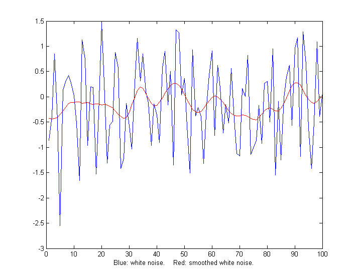
second. Here's a simple example of fastsmooth demonstrating the
effect on white noise (graphic).
x=1:100;
y=randn(size(x));
plot(x,y,x,fastsmooth(y,5,3,1),'r')
xlabel('Blue: white noise. Red: smoothed
white noise.')
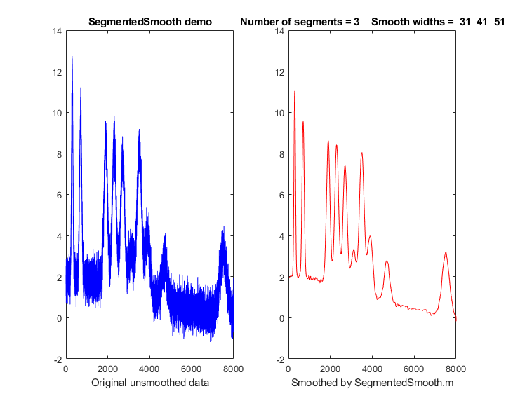 SegmentedSmooth.m, illustrated
on the right, is a segmented version
of fastsmooth, which applies different smooth widths to
different segments of the signal. The
syntax is the same as fastsmooth.m, except that
the second input argument "smoothwidths" can be a vector: SmoothY = SegmentedSmooth (Y,
smoothwidths, type, ends).
The function divides Y into a number of equal-length regions
defined by the length of the vector 'smoothwidths', then smooths
each region with a smooth of type 'type' and width defined by
the elements of vector 'smoothwidths'. In the graphic
example in the figure on the right, smoothwidths=[31 52 91],
which divides up the signal into three equal regions and smooths
the first region with smoothwidth 31, the second with
smoothwidth 51, and the last with smoothwidth 91. Any number of smooth widths and sequence of smooth
widths can be used. Type "help
SegmentedSmooth" for other examples. The demonstration script DemoSegmentedSmooth.m shows
the operation with signal (DemoSegmentedSmooth.mat)
consisting of noisy variable-width peaks that get progressively
wider, like the figure on the right. If the peak widths increase
or decrease regularly across the signal, you can calculate the
smoothwidths vector by giving only the number of segments
("NumSegments") , the first value, "startw", and the last value,
"endw", like so:
SegmentedSmooth.m, illustrated
on the right, is a segmented version
of fastsmooth, which applies different smooth widths to
different segments of the signal. The
syntax is the same as fastsmooth.m, except that
the second input argument "smoothwidths" can be a vector: SmoothY = SegmentedSmooth (Y,
smoothwidths, type, ends).
The function divides Y into a number of equal-length regions
defined by the length of the vector 'smoothwidths', then smooths
each region with a smooth of type 'type' and width defined by
the elements of vector 'smoothwidths'. In the graphic
example in the figure on the right, smoothwidths=[31 52 91],
which divides up the signal into three equal regions and smooths
the first region with smoothwidth 31, the second with
smoothwidth 51, and the last with smoothwidth 91. Any number of smooth widths and sequence of smooth
widths can be used. Type "help
SegmentedSmooth" for other examples. The demonstration script DemoSegmentedSmooth.m shows
the operation with signal (DemoSegmentedSmooth.mat)
consisting of noisy variable-width peaks that get progressively
wider, like the figure on the right. If the peak widths increase
or decrease regularly across the signal, you can calculate the
smoothwidths vector by giving only the number of segments
("NumSegments") , the first value, "startw", and the last value,
"endw", like so:
wstep=(endw-startw)/NumSegments;
smoothwidths=startw:wstep:endw;
The Savitzky-Golay method is ideal for computing smoothed derivatives because it combines differentiation with the right kind of smoothing. The Matlab signal processing program iSignal, or its Octave version isignaloctave, uses this approach. Diederick has published a Savitzky-Golay smooth function in Matlab, which you can download from the Matlab File Exchange. It's included in the iSignal function. Greg Pittam has published a modification of the fastsmooth function that tolerates NaNs ("Not a Number") in the data file (nanfastsmooth(Y,w,type,tol)) and a version for smoothing angle data (nanfastsmoothAngle(Y,w,type,tol)).
 SmoothWidthTest.m is a
demonstration script that uses the fastsmooth function to
demonstrate the effect of smoothing on peak height, noise, and
signal-to-noise ratio of a peak. You can change the peak shape
in line 7, the smooth type in line 8, and the noise in line 9. A
typical result for a Gaussian peak with white noise smoothed
with a pseudo-Gaussian smooth is shown on the left. Here, as it
is for most peak shapes, the optimal signal-to-noise ratio
occurs at a smooth ratio of about 0.8. However, that optimum
corresponds to a significant reduction
in the peak height, which could be a
problem. A smooth width about half the width of the original unsmoothed peak produces less
distortion of the peak but still achieves a reasonable noise
reduction. SmoothVsCurvefit.m
is a similar script, but is also compares curve fitting as an alternative
method to measure the peak height without
smoothing.
SmoothWidthTest.m is a
demonstration script that uses the fastsmooth function to
demonstrate the effect of smoothing on peak height, noise, and
signal-to-noise ratio of a peak. You can change the peak shape
in line 7, the smooth type in line 8, and the noise in line 9. A
typical result for a Gaussian peak with white noise smoothed
with a pseudo-Gaussian smooth is shown on the left. Here, as it
is for most peak shapes, the optimal signal-to-noise ratio
occurs at a smooth ratio of about 0.8. However, that optimum
corresponds to a significant reduction
in the peak height, which could be a
problem. A smooth width about half the width of the original unsmoothed peak produces less
distortion of the peak but still achieves a reasonable noise
reduction. SmoothVsCurvefit.m
is a similar script, but is also compares curve fitting as an alternative
method to measure the peak height without
smoothing.
This effect is explored more completely by the text below, which shows an experiment in Matlab or Octave that creates a Gaussian peak, smooths it, compares the smoothed and unsmoothed version, then uses the max(), halfwidth(), and trapz() functions to print out the peak height, halfwidth, and area. (max and trapz are both built-in functions in Matlab and Octave, but you have to download halfwidth.m. To learn more about these functions, type "help" followed by the function name).
x=[0:.1:10]';
y=exp(-(x-5).^2);
plot(x,y)
ysmoothed=fastsmooth(y,11,3,1);
plot(x,y,x,ysmoothed,'r')
disp([max(y) halfwidth(x,y,5) trapz(x,y)])
disp([max(ysmoothed) halfwidth(x,ysmoothed,5)
trapz(x,ysmoothed)])
1
1.6662 1.7725
0.78442
2.1327 1.7725
These
results
show that smoothing reduces the peak
height (from 1 to 0.784) and increases the peak
width (from 1.66 to 2.13), but has no effect on the peak
area, as long as you measure the total
area under the broadened peak.
Smoothing is useful if the signal
is contaminated by non-normal noise such as sharp spikes or if
the peak height, position, or width are measured by simple
methods, but there is no need to smooth the data if the noise is
white and the peak parameters are measured by least-squares
methods, because the least-squares
results obtained on the unsmoothed data will be more
accurate (see CurveFittingC.html#Smoothing).
The Matlab/Octave user-defined function condense.m, condense(y,n), returns a
condensed version of y in which each group of n points is replaced by its average, reducing the
length of y
by the factor n. This operation is also called "bunching". (For
x,y data sets,
use this function on both independent variable x and dependent variable y so that the features of y will appear at the same x values).
The Matlab/Octave user-defined function medianfilter.m, medianfilter(y,w), performs a median-based filter operation that replaces each value of y with the median of w adjacent points (which must be a positive integer). killspikes.m is a threshold-based filter for eliminating narrow spike artifacts. The syntax is fy= killspikes(x, y, threshold, width). Each time it finds a positive or negative jump in the data between y(n) and y(n+1) that exceeds "threshold", it replaces the next "width" points of data with a linearly interpolated segment spanning x(n) to x(n+width+1), See killspikesdemo. Type "help killspikes" at the command prompt.
ProcessSignal is a Matlab/Octave
command-line function that performs smoothing and
differentiation on the time-series data set x,y (column or row
vectors). It can employ all the types of smoothing
described above. Type "help ProcessSignal". Returns the
processed signal as a vector that has the same shape as x,
regardless of the shape of y. The syntax is Processed=ProcessSignal(x, y,
DerivativeMode, w, type, ends, Sharpen, factor1, factor2,
SlewRate, MedianWidth)
Real-time
smoothing in Matlab is discussed in Appendix Y.
Live script for smoothing
Here is a
Matlab Live
Script (download link: DataSmoothing.mlx) for
performing several types of smoothing applied to
experimental data stored on disk. It can perform:
Clicking
the "Open data file" button in line 1 opens a file
browser, allowing you to navigate to your data file (in .csv
or .xlsx format; the script assumes that your x,y data are
in the first two columns). All the variables and settings
appear in the Matlab workspace as usual; the finished
smoothed data are in the vector "sy".

The script has several interactive controls.
The startpc and endpc sliders in lines 7 and 8
allow you to select which portion of the data range to process,
from 0% to 100% of the total range of the data file.
The SmoothType drop-down
menu in line 13 selects the smoothing algorithm; each
has one or more controls specific to that type in lines 16 to
30. The first choice is the recursive sliding average (fastsmooth.m)
algorithm explained above. The smooth width and number of passes
are controlled by the sliders in lines 16 and 17. Each The other
controls are explained in the accompanying comment lines (in
green). Fourier filtering, Savitsky-Golay and wavelet denoising
are topics that will be explained in later sections.
The PlotBeforeAndAfter checkbox in
line 3 gives you the option of plotting the original signal (in
black) along with the processed signal (in red).
The FrequencySpectra checkbox in line 4 allows you to show the frequency spectrum of the original and/or processed signals (see HarmonicAnalysis.html). Note: to view the graphic plots to the right of the code, as shown above, right-click on the empty space on the right and select "Disable synchronous scrolling".
Smoothing in
iSignal
iSignal is an interactive function for Matlab that performs smoothing for time-series signals using all the algorithms discussed above, including the Savitzky-Golay smooth, segmented smooth, a median filter, and a condense (bunching) function, with keystrokes that allow you to adjust the smoothing parameters continuously while observing the effect on your signal instantly, making it easy to observe how different types and amounts of smoothing effect noise and signal, such as the height, width, and areas of peaks. Other functions include differentiation, peak sharpening, interpolation, least-squares peak measurement, and a frequency spectrum mode that shows how smoothing and other functions can change the frequency spectrum of your signals. The simple script "iSignalDeltaTest" demonstrates the frequency response of iSignal's smoothing functions by applying them to a single-point spike, allowing you to change the smooth type and the smooth width to see how the the frequency response changes. View the code here or download the ZIP file with sample data for testing.
iSignal for Matlab, showing the smoothing of a signal (upper panel) that is contaminated by a strong parasitic oscillation. The frequency spectrum is shown in the lower panel. As the smooth width increases, the oscillation is suppressed and the signal peaks come into view. Too much smoothing, however, broadens and shortens the peaks. Click to view larger figure.
You
try it: Here's an example of a very noisy signal with lots
of high-frequency (blue) noise totally obscuring a
perfectly good peak in the center at x=150, height=1e-4;
SNR=90. First, download NoisySignal
into the Matlab path, then execute these statements:
>> load NoisySignal
>> isignal(x,y);
Use the A and Z keys to increase and decrease
the smooth width, and the S key to cycle through the
available smooth types. Hint: use the Gaussian smooth and keep
increasing the smooth width until the peak shows.
Note: you can right-click on any of the m-file links on this site and select Save Link As... to download them to your computer for use within Matlab. Unfortunately, iSignal does not currently work in Octave.
An earlier version of his page is available in French, at http://www.besteonderdelen.nl/blog/?p=4169, courtesy of Natalie Harmann and Anna Chekovsky.
Last updated April,
2023. This page is part of "A
Pragmatic Introduction to Signal Processing", created and maintained by Prof. Tom O'Haver ,
Department of Chemistry and Biochemistry, The University of
Maryland at College Park. Comments, suggestions, bug reports,
and questions should be directed to Prof. O'Haver at toh@umd.edu.
Unique visits since May 17, 2008:

