Making predictive maps from RSF’s
Resource Selection Functions, Part IV
Elie Gurarie
2019-12-02
Goals: Learning to make predictions from a fitted RSF, including making a “habitat suitability” map
Making a predictive map of an RSF is - in principle - straightforward:
- Take the model you want to predict
- Obtain raster stack with all of the available covariates
- Compute the values of the RSF for the covariates
- Place them in a raster of the same properties as the brick
The details - as usual - are in the weeds and have more to do with managing the data and being patient than anything else.
The following packages are the only ones we’ll need:
pcks <- c("glmmTMB", "raster", "plyr", "magrittr")
a <- sapply(pcks, require, character = TRUE)
1. Obtain the RSF
The model we’ll use is the random slope model selected from the last primer. Recall that it includes EOSD class, road density, 1st and 2nd order elevation terms, and random slopes on the elevation and road density.
The RSF processed data we saved:
load("_data/hayriver_RSF.rda")
hr <- hayriver.RSF
And the model fitting is as follows:
require(glmmTMB)
hayriver.model <- glmmTMB(formula = Used ~ EOSD.class + scale(Road.Density) + scale(poly(DEM,
    2)) - 1 + (scale(Road.Density) + scale(DEM) | nick_name),
    data = hr, family = "binomial", ziformula = ~0, dispformula = ~1)
The predict function
There are a lot of coefficients to this model:
hayriver.model## Formula:
## Used ~ EOSD.class + scale(Road.Density) + scale(poly(DEM, 2)) -
## 1 + (scale(Road.Density) + scale(DEM) | nick_name)
## Data: hr
## AIC BIC logLik df.resid
## 3569.329 3748.803 -1759.665 9666
## Random-effects (co)variances:
##
## Conditional model:
## Groups Name Std.Dev. Corr
## nick_name (Intercept) 1.322
## scale(Road.Density) 0.428 0.05
## scale(DEM) 2.512 0.18 -0.62
##
## Number of obs: 9691 / Conditional model: nick_name, 13
##
## Fixed Effects:
##
## Conditional model:
## EOSD.classConiferous-dense EOSD.classBroadleaf-dense
## 0.5372 -2.1004
## EOSD.classBroadleaf-open EOSD.classBryoids
## -2.1642 -0.9076
## EOSD.classConiferous-open EOSD.classConiferous-sparse
## 0.6946 0.0418
## EOSD.classDeveloped EOSD.classMixedwood-dense
## -20.3771 -0.7631
## EOSD.classMixedwood-open EOSD.classRecent Burn
## 0.5289 -0.1616
## EOSD.classShrub Low EOSD.classShrub Tall
## -0.3068 -13.9791
## EOSD.classWater EOSD.classWetland-herb
## -1.8660 0.2929
## EOSD.classWetland-shrub EOSD.classWetland-treed
## 0.2788 0.8619
## scale(Road.Density) scale(poly(DEM, 2))1
## 0.1288 -3.0336
## scale(poly(DEM, 2))2
## -4.7070Recall that the model we fit is a logistic model, but the (typical) definition of a resource selection model is a normalized numerator of that model, i.e.:
\[w_i(x, \beta) = \exp(\beta_0 + \beta_1 x_1 + \beta_2 x_2 + \beta_3 x_3 + ...)\]
The “normalization” - really just a way to constrain the range of these values (which can be quite large) - can either constrain the RSF to being between 0 to 1 or - somewhat more strictly - to integrating (or summing) to one over the entire domain, which leads to very small absolute values. These details don’t matter so much, since the interpretation is always of relative “suitability” of habitat, and the intercept itself is arbitrarily set by the number of available points.
It is easy to generate predictions from this model (and any fitted model) using the predict function. By default, this function returns the linear predictor (i.e.: the sum \(\beta_0 + \beta_1 x_1 + \beta_2 x_2 + \beta_3 x_3 + ...\)). The requirement is to have new data formatted identically to the orignial data used to fit the model. For example, to see what the elevation preference profile might look like, you can create a dummy data frame in the open coniferous habitat type in areas with zero road densities. We set elevations that cover the range of available elevations (140-800 m):
DEM = 140:900
newdata <- data.frame(EOSD.class = "Coniferous-open", DEM, Road.Density = 0, nick_name = "dummy")
RSF.prediction <- predict(hayriver.model, newdata = newdata, allow.new.levels=TRUE)
plot(newdata$DEM, RSF.prediction, type = "l", ylab = "linear predictor")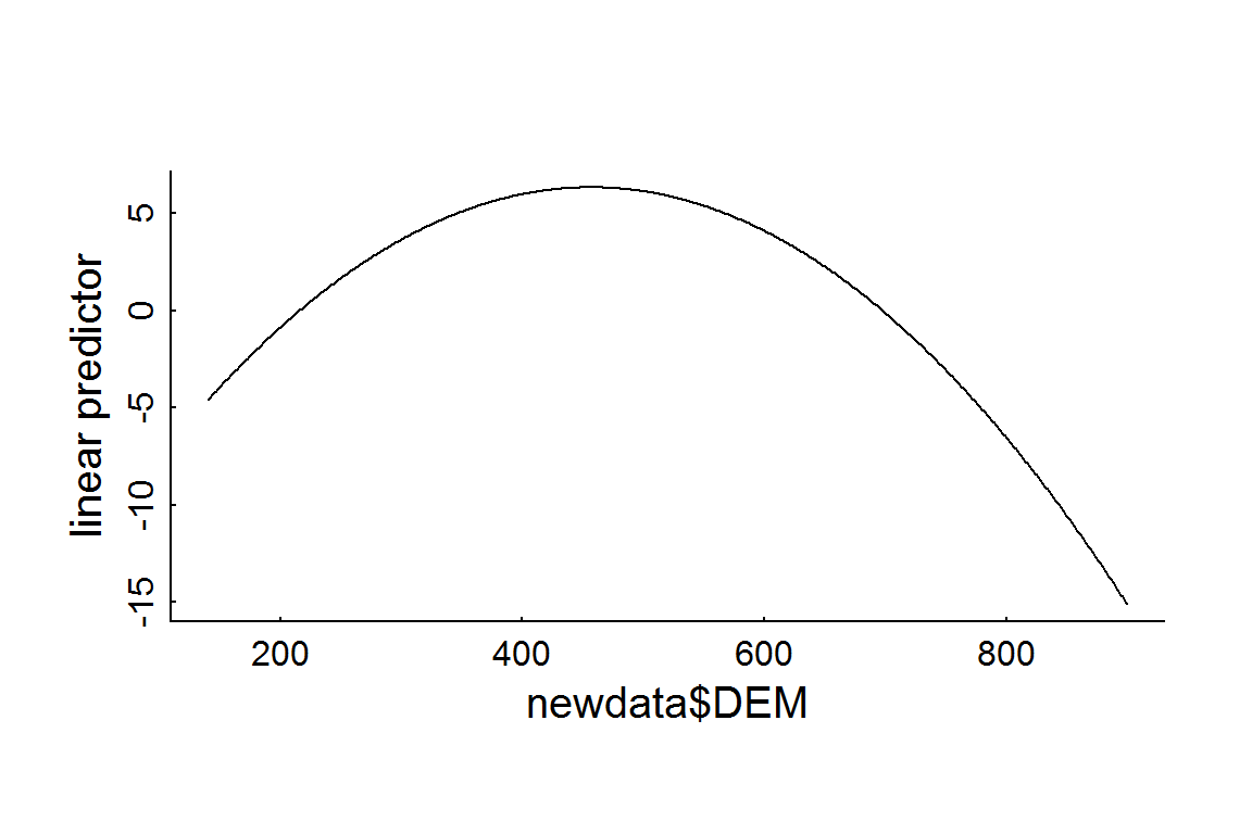
Note that that this plot is in the log-odds scale. According to this fitted model, the peak preferred elevation is DEM[which.max(RSF.prediction)] = 457 m. To obtain the RSF itself, you simply take the exponent (and - somehow - normalize), e.g:
plot(newdata$DEM, exp(RSF.prediction)/max(exp(RSF.prediction)), type = "l", ylab = "RSF")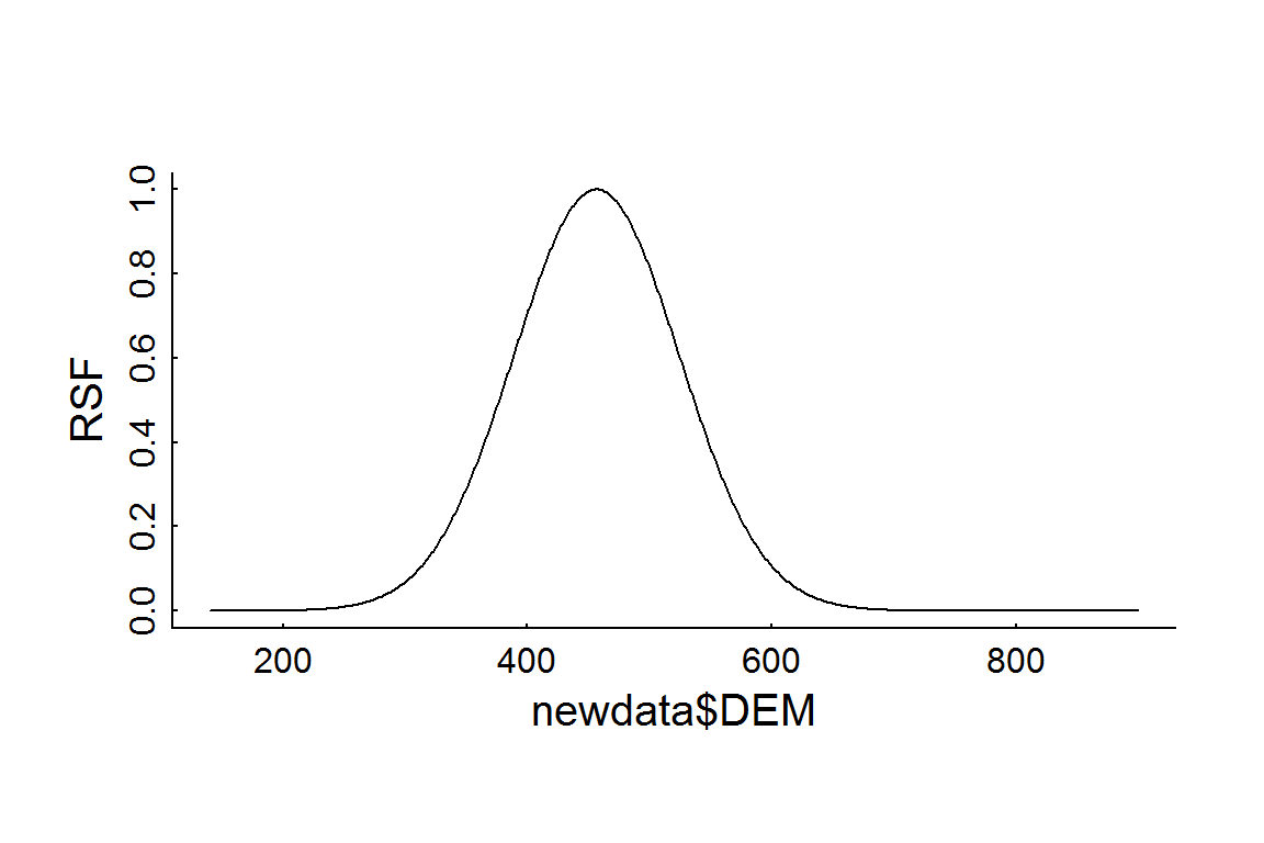
The following code obtains fits and standard errors and plots those predictions with confidence (or prediction) intervals, which are obtained by adding the se.fit = TRUE flag to the predict function:
RSF.prediction.se <- predict(hayriver.model, newdata = newdata, allow.new.levels=TRUE, se.fit = TRUE)
RSF.prediction.df <- with(RSF.prediction.se, data.frame(DEM = newdata$DEM, rsf.hat = exp(fit)/max(exp(fit)),
                                                        CI.low = exp(fit - 2*se.fit)/max(exp(fit)),
                                                        CI.high = exp(fit + 2*se.fit)/max(exp(fit))))

with(RSF.prediction.df, {
     plot(DEM, rsf.hat, lwd = 2, type = "l", log = "y", ylim = c(1e-5, 100), ylab = "RSF function")
      lines(DEM, CI.low, col = "darkgrey", lwd = 2)
      lines(DEM, CI.high, col = "darkgrey", lwd = 2)
})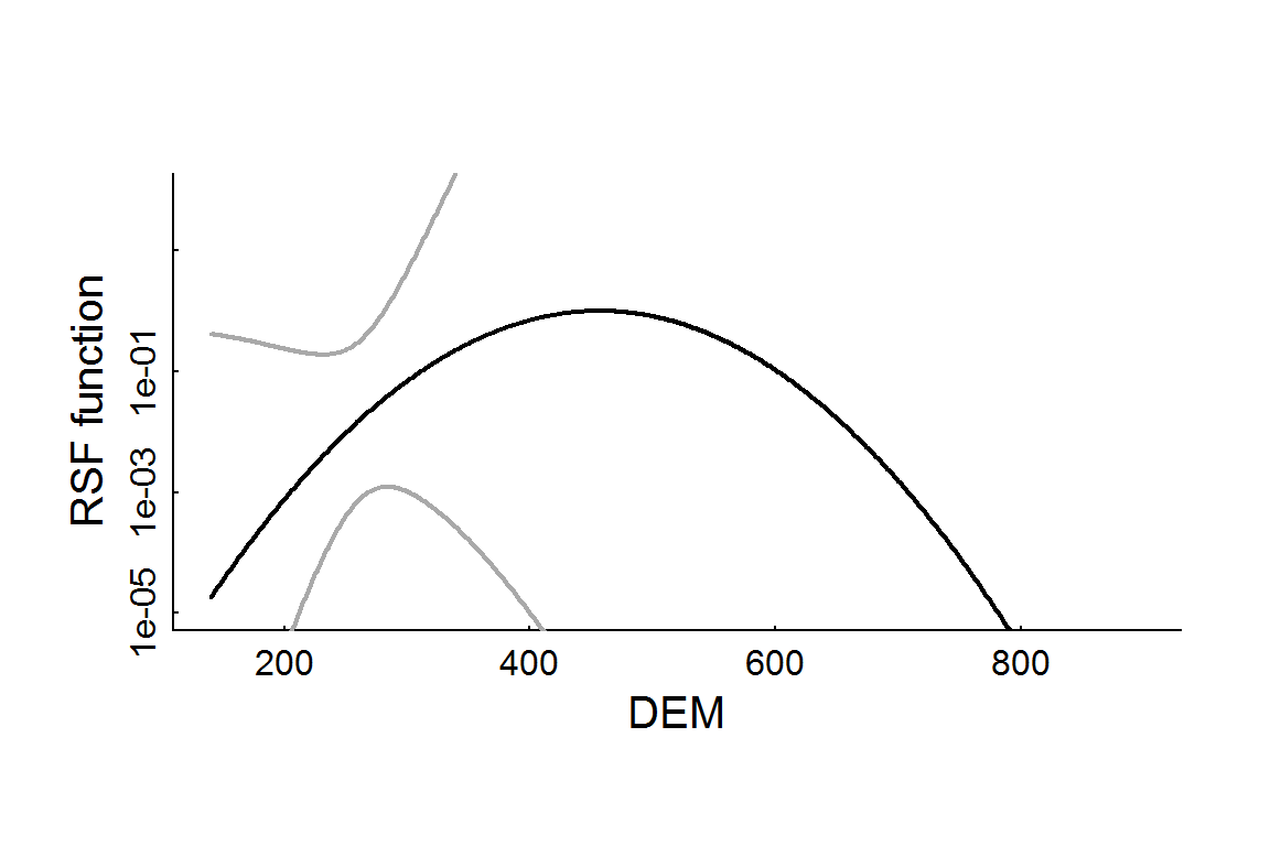
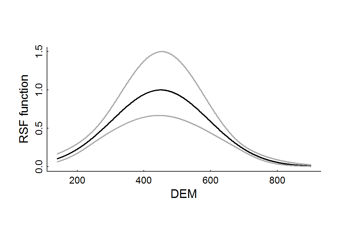
The confidence intervals are EXTREMELY wide for this model (it even had to be plotted on a log-scale). This is because it is a mixed model, which is less likely to overfit. For comparison, here is a “straight” logistic regression, and the resulting elevation RSF profile:
hayriver.glm <- glm(formula = Used ~ EOSD.class + scale(Road.Density) + scale(poly(DEM,
    2)) - 1, data = hr, family = "binomial")

RSF.glm.se <- predict(hayriver.glm, newdata = newdata, allow.new.levels=TRUE, se.fit = TRUE)
RSF.glm.df <- with(RSF.glm.se, data.frame(DEM = newdata$DEM, rsf.hat = exp(fit)/max(exp(fit)),
                                                        CI.low = exp(fit - 2*se.fit)/max(exp(fit)),
                                                        CI.high = exp(fit + 2*se.fit)/max(exp(fit))))

with(RSF.glm.df, {
     plot(DEM, rsf.hat, lwd = 2, type = "l", ylim = c(0,1.5), ylab = "RSF function")
      lines(DEM, CI.low, col = "darkgrey", lwd = 2)
      lines(DEM, CI.high, col = "darkgrey", lwd = 2)
})
2. Load the brick and extract values
Now, we have to load the brick that we generated two primers ago in order to extract the variables for the movement data. Recall - this is a very large object (250 Mb - just for the Hay River portion of the data) and it will - hopefully - be stored somewhere on your computer. We used the tif format to save it to save space, but that means we also need to rename the layers. Thus:
Covar.brick <- brick("c:/eli/caribou/NWT/data/RSF_brick_v2.tif")
names(Covar.brick) <- c("EOSD", "Road Density", "DEM")
plot(Covar.brick, nc = 3)
For the sake of tractability, we will crop this brick to a somewhat smaller 50 x 50 km range
Covar.brick.small <- crop(Covar.brick,
                        extent(c(-2.6e5,-2.1e5, 22.5e5, 23e5)))
plot(Covar.brick.small, nc = 3)
The values function takes ALL of the data in this raster and conveniently converts to a matrix:
Covar.brick.values <- values(Covar.brick.small)
head(Covar.brick.values)
## EOSD Road.Density DEM
## [1,] 231 0 280.3086
## [2,] 231 0 280.4015
## [3,] 231 0 280.5112
## [4,] 231 0 280.7028
## [5,] 222 0 280.8944
## [6,] 222 0 281.0860Because in our model we fitted to the discrete, named EOSD class, we have to match the EOSD values in the raster to the classes in the original EOSD file. One way to do that is to extract the unique EOSD - EOSD.class combinations from the analysis data frame and perform a merge. NOTE, however, that merge often (and mysteriously) rearranges the order of the items in a given data frame. ALSO, very important to add the all.x = TRUE tag to merge, otherwise missing data will simply be eliminated from . We therefore need to add a row ID column and reorder the merged data frame appropriately. Also, we need to add a “dummy” nick_name column. Thus:
EOSD.table <- unique(hr[,c("EOSD","EOSD.class")])
Covar.brick.values <- Covar.brick.values %>% data.frame %>%
  mutate(rid = 1:length(EOSD), nick_name = "dummy") %>%
  merge(EOSD.table, all.x = TRUE) %>% arrange(rid)
str(Covar.brick.values)
## 'data.frame': 2777222 obs. of 6 variables:
## $ EOSD : num 231 231 231 231 222 222 222 222 231 231 ...
## $ Road.Density: num 0 0 0 0 0 0 0 0 0 0 ...
## $ DEM : num 280 280 281 281 281 ...
## $ rid : int 1 2 3 4 5 6 7 8 9 10 ...
## $ nick_name : chr "dummy" "dummy" "dummy" "dummy" ...
## $ EOSD.class : Factor w/ 20 levels "Broadleaf-dense",..: 10 10 10 10 2 2 2 2 10 10 ...The data are now ready to perform the prediction on.
3. Predict over a raster
One issue with just running prediction on the complete covariate data frame is that data are not available for ALL the rows. The allow.new.levels = TRUE flag is necessary to not get errors for those habitat types which might not appear in the subsetted data frame.
system.time(hayriver.prediction <- predict(hayriver.model, newdata = Covar.brick.values, allow.new.levels=TRUE))## user system elapsed
## 94.58 32.56 129.76str(hayriver.prediction)## num [1:2777222] 2.91 2.87 2.82 2.74 1.25 ...Terrific! We now have a vector with all the predictions (and of the correct length).
4. Fill a raster with these predictions
We can now fill a new raster level with these values for the linear predictor:
logRSF.layer <- Covar.brick.small[[1]] %>% setValues(hayriver.prediction)
plot(logRSF.layer)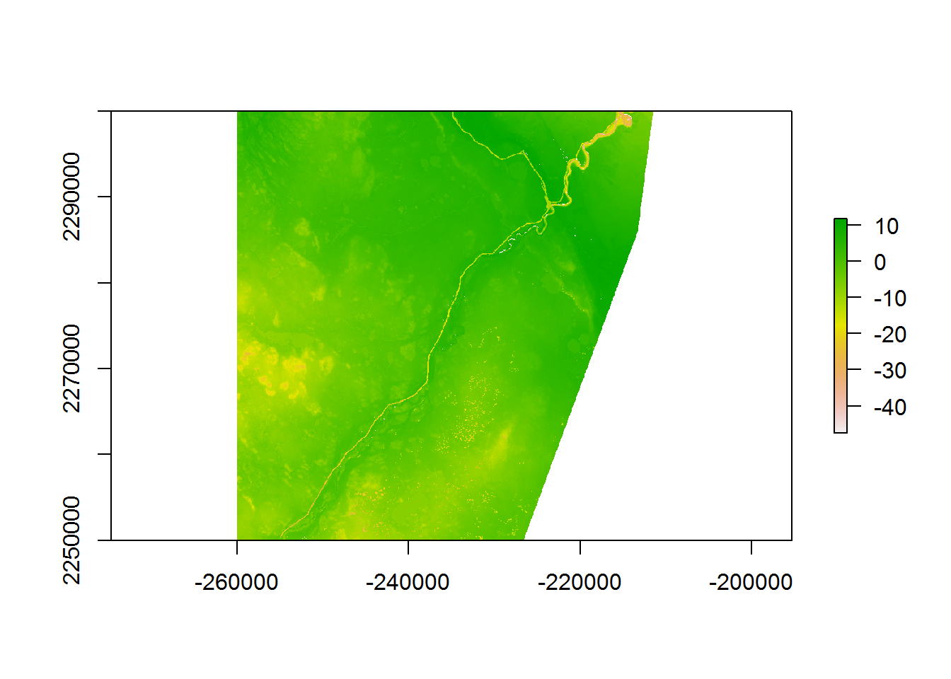
Or in terms of the actual RSF numerator:
RSF.layer <- exp(logRSF.layer)/max(values(exp(logRSF.layer)), na.rm = TRUE)
plot(RSF.layer)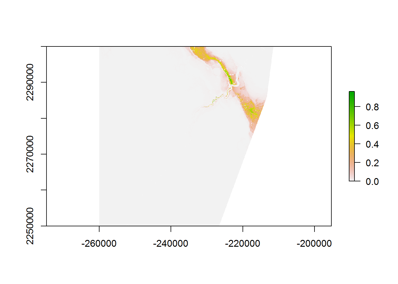
But in light of the extreme magnitude and contrast in these values, neither of these figures is very satisfying. In a recent review of mapping RSF’s (Morris et al. 2016)1, the authors explicitly recommend against the display of continuous RSF surfaces because there is no established method for testing the predictive accuracy of a continuous RSF surface. A a widely used approach is to map equal area divisions (typically - 10). To compute these, we rely on two fundamental base R functions: quantile - which breaks data into any number of percentiles - and cut - which converts continuous data to factors. I’ll do a 20 equal area cut as an example here:
(breaks <- quantile(hayriver.prediction, seq(0,1,1/10), na.rm = TRUE))## 0% 10% 20% 30% 40% 50%
## -48.7425327 -8.0234728 -5.5557369 -3.6552487 -1.9573867 -0.3996516
## 60% 70% 80% 90% 100%
## 1.1629441 3.1154503 4.5878430 6.2684881 11.8441931hayriver.RSF.discrete <- cut(hayriver.prediction, breaks = breaks, labels = 1:10)
RSF.class <- RSF.layer %>% setValues(hayriver.RSF.discrete)Now you can plot a good, high-contrast map of the RSF’s, with 10 clear categories
require(gplots)
plot(RSF.class, col = rich.colors(10))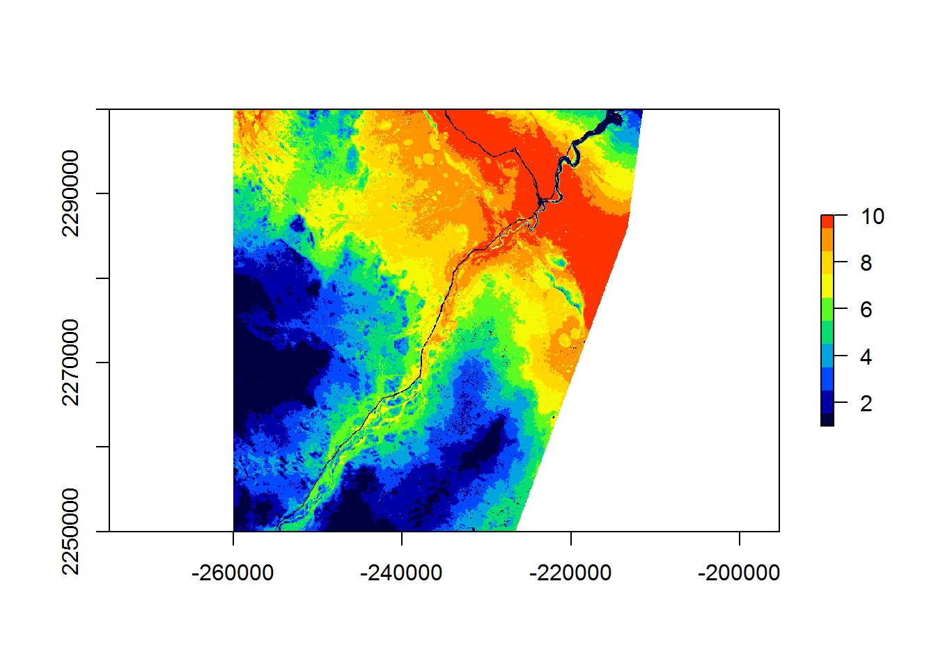
Overall, clear patterns emerge, including the strong avoidance of the main road (and river) going through the middle of this portion of the landscape and a preference for the more intermediate elevations.
5. Post-hoc analysis of landcapes
One way to communicate the on-the-ground features of this break-down is to simply compare the variables across the habitat classes. Below, I perform this analysis for an RSF of the entire Hay River lowlands area. This is also an opportunity to review all the steps of the RSF mapping. Note that in this example - to save time - I fit only a glm without worrying about random effects.
##. load packages
pcks <- c("glmmTMB", "raster", "plyr", "magrittr", "ggplot2", "gplots")
a <- sapply(pcks, require, character = TRUE)
a. Load data and fit model
load("_data/hayriver_RSF.rda")
hr <- hayriver.RSF
hayriver.glm <- glm(formula = Used ~ EOSD.class + scale(Road.Density) +
                      scale(poly(DEM,2)) - 1, data = hr, family = "binomial")
b. Load and prep raster
Covar.brick <- brick("c:/eli/caribou/NWT/data/RSF_brick_v2.tif")
names(Covar.brick) <- c("EOSD", "Road Density", "DEM")
Covar.brick.values <- values(Covar.brick)

EOSD.table <- unique(hr[,c("EOSD","EOSD.class")])
Covar.brick.values <- data.frame(Covar.brick.values,
                                 EOSD.class =  EOSD.table$EOSD.class[match(Covar.brick.values[, "EOSD"], EOSD.table$EOSD)])
c. make predictions from fitted model
hr.glm.prediction <- predict(hayriver.glm,
                             newdata = Covar.brick.values[!is.na(Covar.brick.values$DEM),],
                             allow.new.levels=TRUE)
d. Merge predictions and discretize
breaks <- quantile(hr.glm.prediction, seq(0,1,1/10), na.rm = TRUE)
hr.glm.RSF.class <- rep(NA, nrow(Covar.brick.values))
hr.glm.RSF.class[!is.na(Covar.brick.values$DEM)] <- cut(hr.glm.prediction, breaks = breaks, labels = 1:10)
RSF.glm.class <- Covar.brick[[1]] %>% setValues(hr.glm.RSF.class)
e. Plot RSF
plot(RSF.glm.class, col = rich.colors(10), maxpixels = 2e6)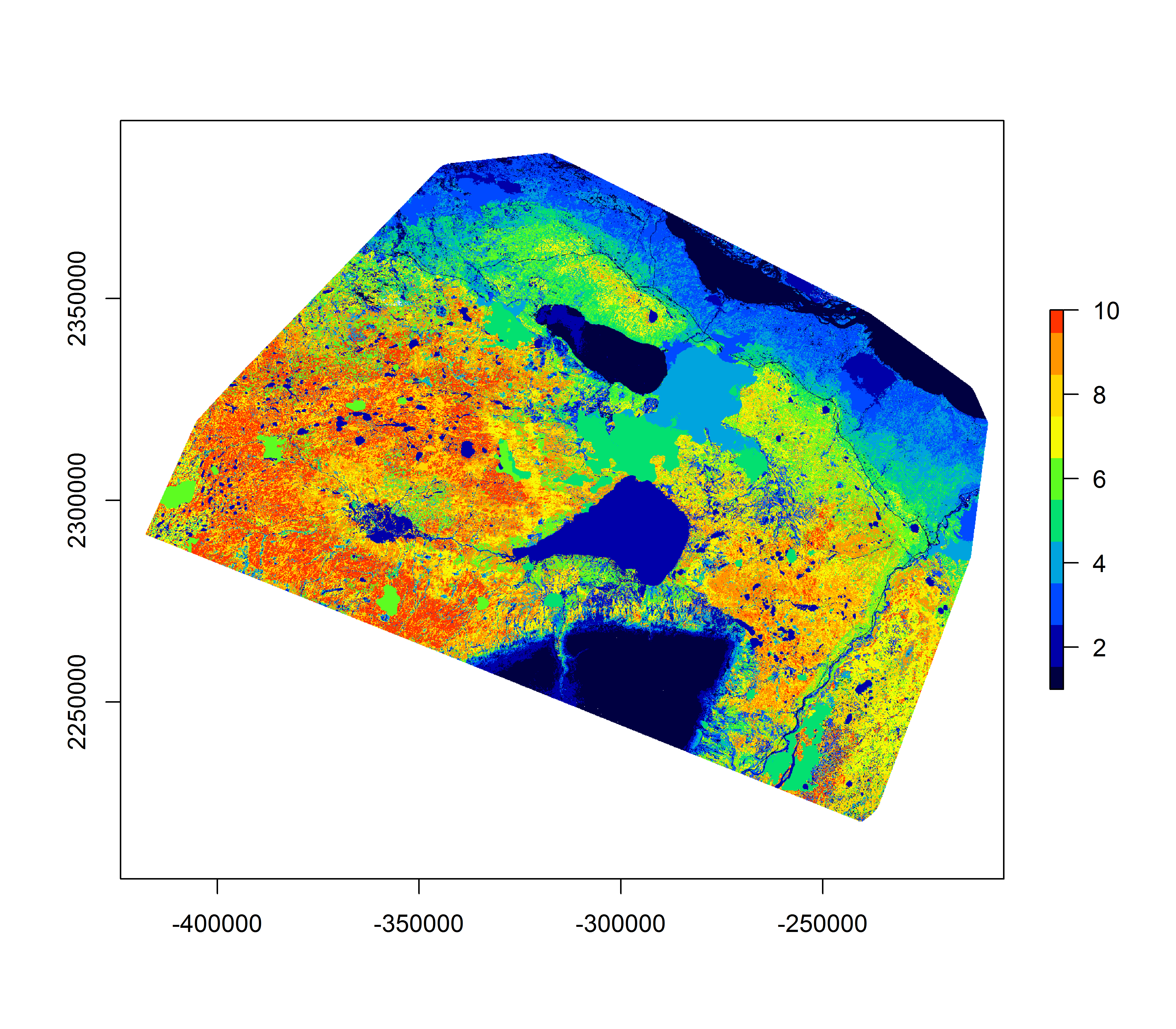
Covar.brick.values$RSF.class <- hr.glm.RSF.classf. Plot covariates against class
DEM vs. RSF class
ddply(Covar.brick.values %>% subset(!is.na(RSF.class)) %>%
        mutate(RSF.class = factor(RSF.class)), "RSF.class", summarize,
      dem.median = median(DEM),
      min = min(DEM, na.rm = TRUE), max = max(DEM, na.rm = TRUE),
      Q1 = quantile(DEM, .025), Q2 = quantile(DEM, .975),
      Q3 = quantile(DEM, .25), Q4 = quantile(DEM, .75)) %>%
  ggplot(aes(RSF.class, dem.median)) +
  geom_linerange(aes(ymin = min, ymax = max), lwd = 2, col = "grey") +
  geom_linerange(aes(ymin = Q1, ymax = Q2), lwd = 4, col = "darkgrey") +
  geom_linerange(aes(ymin = Q3, ymax = Q4), lwd = 8) +
  geom_point(col = "lightblue", cex = 2) + ggtitle("Elevation v. RSF class")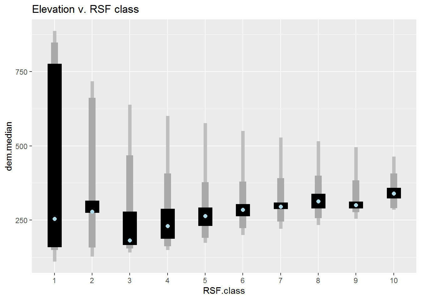
Road Density vs. RSF class
 ddply(Covar.brick.values %>% subset(!is.na(RSF.class)) %>%
        mutate(RSF.class = factor(RSF.class)), "RSF.class", summarize,
      Road.Density.median = median(Road.Density),
      min = min(Road.Density, na.rm = TRUE), max = max(Road.Density, na.rm = TRUE),
      Q1 = quantile(Road.Density, .025), Q2 = quantile(Road.Density, .975),
      Q3 = quantile(Road.Density, .25), Q4 = quantile(Road.Density, .75)) %>%
  ggplot(aes(RSF.class, Road.Density.median)) +
  geom_linerange(aes(ymin = min, ymax = max), lwd = 2, col = "grey") +
  geom_linerange(aes(ymin = Q1, ymax = Q2), lwd = 4, col = "darkgrey") +
  geom_linerange(aes(ymin = Q3, ymax = Q4), lwd = 8) +
  geom_point(col = "lightblue", cex = 2) + ggtitle("Road Density v. RSF class")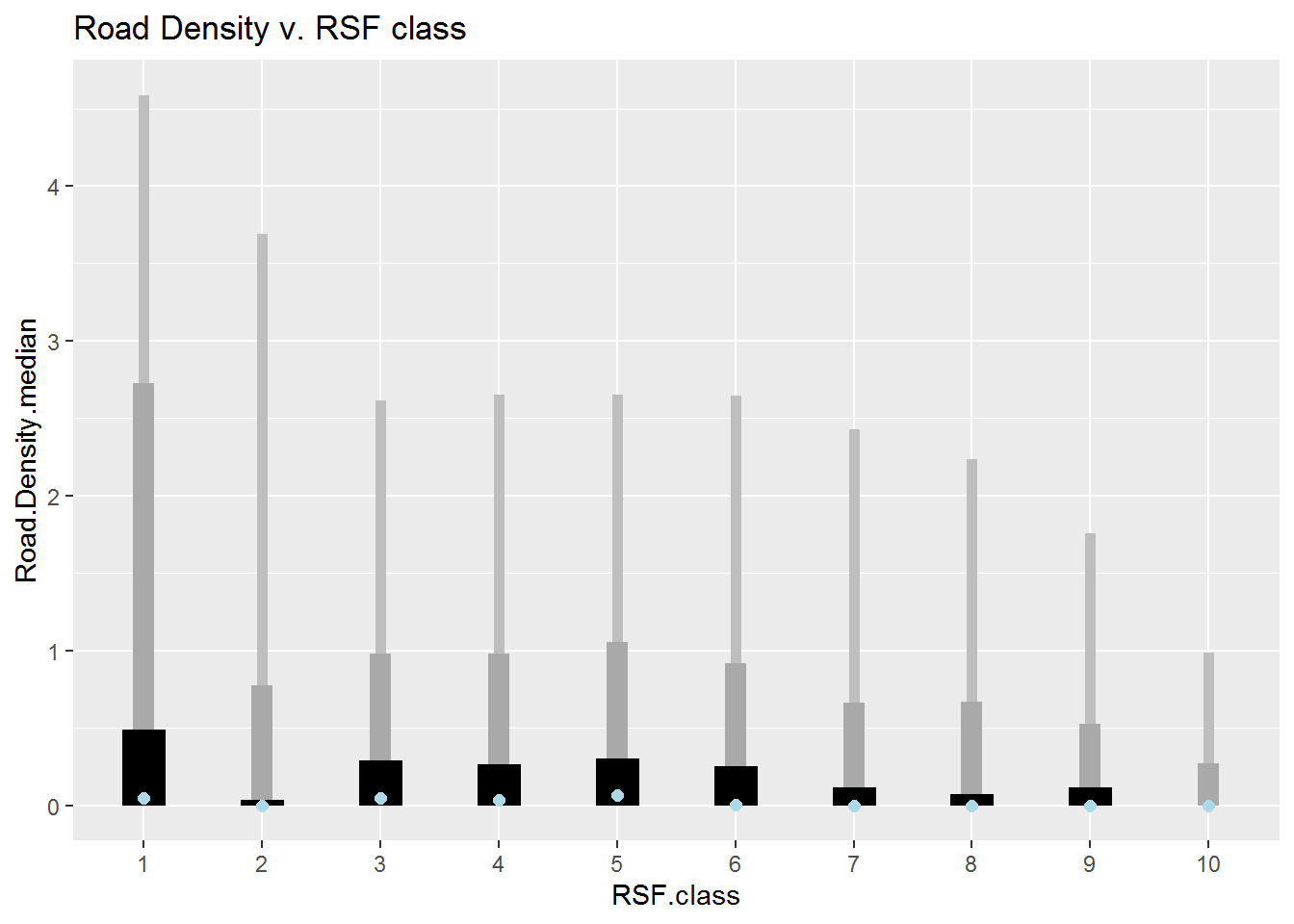
Habitat Type vs. RSF Class.
Note the use of the powerful and too obscure mosaicplot function, which is the absolute best tool in my opinion for plotting categorical variables against categorical variables.
palette(rich.colors(10))
par(cex.axis = 0.7, mar = c(8,2,0,1))
t <- with(Covar.brick.values %>% droplevels, table(RSF.class, EOSD.class))
EOSD.scores <- ddply(Covar.brick.values, "EOSD.class", summarize, RSF.mean = mean(RSF.class, na.rm = TRUE))
eosd.ordered <- arrange(EOSD.scores, RSF.mean)$EOSD.class %>% na.omit %>% as.character
t.df <- as.data.frame.matrix(t)
tt.df <- t(t.df[,eosd.ordered])
par(cex.axis = 0.7, mar = c(2,0,4,2), oma = c(0,2,0,0))
mosaicplot(tt.df, col = 1:10, las = 2, off = 5, bor = NA, main = "")
legend("left", fill = 1:10, title = "RSF class", legend = 1:10, cex = 0.7)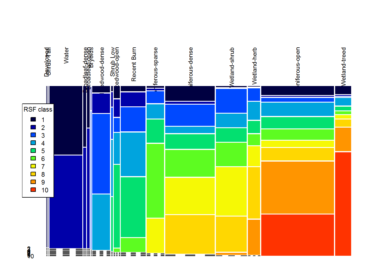
These plots are pretty informative. You can see, for example, that class 10 (the best habitat) is ENTIRELY in the Wetland-treed and Coniferous Open habitat, that the class 9 & 10 elevations are all between about 270-480 m, and that most of the higher road density locations are in the lowest reference classes.
Bonus: Interactive RSF map!
It can be illuminating also to look at how this RSF prediction maps directly on top of sattelite imagery:
require(mapview)
mapview(RSF.glm.class, map.types = "Esri.WorldImagery")
Morris, L.R., Proffitt, K.M. and Blackburn, J.K., 2016. Mapping resource selection functions in wildlife studies: Concerns and recommendations. Applied Geography, 76, pp.173-183.↩︎