Anthropogenic Disturbance: Densities and Distances from Lines and Polygons
Elie Gurarie and Laura Berman
2019-04-16
This is a primer for analyzing anthropogenic disturbances in the Northwest Territories, Canada. The main goals are to learn how to work with linear features and polygons and generate rasters of densities and distances.
1 Linear features
“Linear features” refers to linear anthropogenic disturbances such as roads, seismic lines, pipelines and railroads. The linear features in our portion of NWT are in this file: BEADlines2015_NWT_corrected_to_NT1_2016:
require(sf)
BEAD.lines <- st_read("_data/BEAD/BEADlines2015_NT1_Bistcho_Calendar_MaxH_Yates_HRL_clip.shp")## Reading layer `BEADlines2015_NT1_Bistcho_Calendar_MaxH_Yates_HRL_clip' from data source `C:\Users\Elie\Box Sync\caribou\NWT\rsf\primers\_data\BEAD\BEADlines2015_NT1_Bistcho_Calendar_MaxH_Yates_HRL_clip.shp' using driver `ESRI Shapefile'
## Simple feature collection with 4063 features and 32 fields
## geometry type: MULTILINESTRING
## dimension: XY
## bbox: xmin: -1299584 ymin: 2381243 xmax: -1048374 ymax: 2673503
## epsg (SRID): NA
## proj4string: +proj=aea +lat_1=50 +lat_2=70 +lat_0=40 +lon_0=-96 +x_0=0 +y_0=0 +datum=NAD83 +units=m +no_defsThis is a simple feature object where each row (or “feature”) is a “multilinestring”:
head(BEAD.lines)## Simple feature collection with 6 features and 32 fields
## geometry type: MULTILINESTRING
## dimension: XY
## bbox: xmin: -1245867 ymin: 2418748 xmax: -1156866 ymax: 2588417
## epsg (SRID): NA
## proj4string: +proj=aea +lat_1=50 +lat_2=70 +lat_0=40 +lon_0=-96 +x_0=0 +y_0=0 +datum=NAD83 +units=m +no_defs
## viewSymbol Class tag30m_201 viewSym15m tagPan15m_ Edit_Date Editor
## 1 V Seismic <NA> <NA> <NA> <NA> <NA>
## 2 V Seismic <NA> <NA> <NA> <NA> <NA>
## 3 V Road <NA> <NA> <NA> <NA> <NA>
## 4 New Seismic <NA> <NA> <NA> <NA> <NA>
## 5 V Seismic <NA> <NA> <NA> <NA> <NA>
## 6 V Road <NA> <NA> <NA> <NA> <NA>
## Phase OID_2011 LS_Path LS_Row LS_Date Comment201 Herd dust dangle
## 1 0 0 0 0 <NA> <NA> <NA> 0 0
## 2 0 0 0 0 <NA> <NA> <NA> 0 0
## 3 0 0 0 0 <NA> <NA> <NA> 0 0
## 4 0 0 0 0 <NA> <NA> <NA> 0 0
## 5 0 0 0 0 <NA> <NA> <NA> 0 0
## 6 0 0 0 0 <NA> <NA> <NA> 0 0
## Verified Initials Vector_ver Comment2_1 Province tempOIDJOI update2014
## 1 <NA> <NA> <NA> <NA> <NA> 0 0
## 2 <NA> <NA> <NA> <NA> <NA> 0 0
## 3 <NA> <NA> <NA> <NA> <NA> 0 0
## 4 <NA> <NA> <NA> <NA> <NA> 0 0
## 5 <NA> <NA> <NA> <NA> <NA> 0 0
## 6 <NA> <NA> <NA> <NA> <NA> 0 0
## tempShort verif2015c verif2015e SplitTool xfer2010to SHAPE_STLe
## 1 0 <NA> <NA> <NA> 0 0
## 2 0 <NA> <NA> <NA> 0 0
## 3 0 <NA> <NA> <NA> 0 0
## 4 0 <NA> <NA> <NA> 0 0
## 5 0 <NA> <NA> <NA> 0 0
## 6 0 <NA> <NA> <NA> 0 0
## Shape_Leng LENGTH Shape_Le_1 geometry
## 1 0 0 344.3527 MULTILINESTRING ((-1161197 ...
## 2 0 0 290.2376 MULTILINESTRING ((-1156866 ...
## 3 0 0 550.7962 MULTILINESTRING ((-1203639 ...
## 4 0 0 910.0200 MULTILINESTRING ((-1245867 ...
## 5 0 0 3740.0593 MULTILINESTRING ((-1197697 ...
## 6 0 0 2449.2499 MULTILINESTRING ((-1194690 ...Here is a plot, with a customized color scheme and legend:
require(scales)
colors <- c("grey", "red", "darkgreen", "darkblue", "orange", "purple")
plot(st_geometry(BEAD.lines), col = colors[BEAD.lines$Class])
legend("bottomleft", fill = colors, legend = levels(BEAD.lines$Class), bty = "n", cex = 0.8)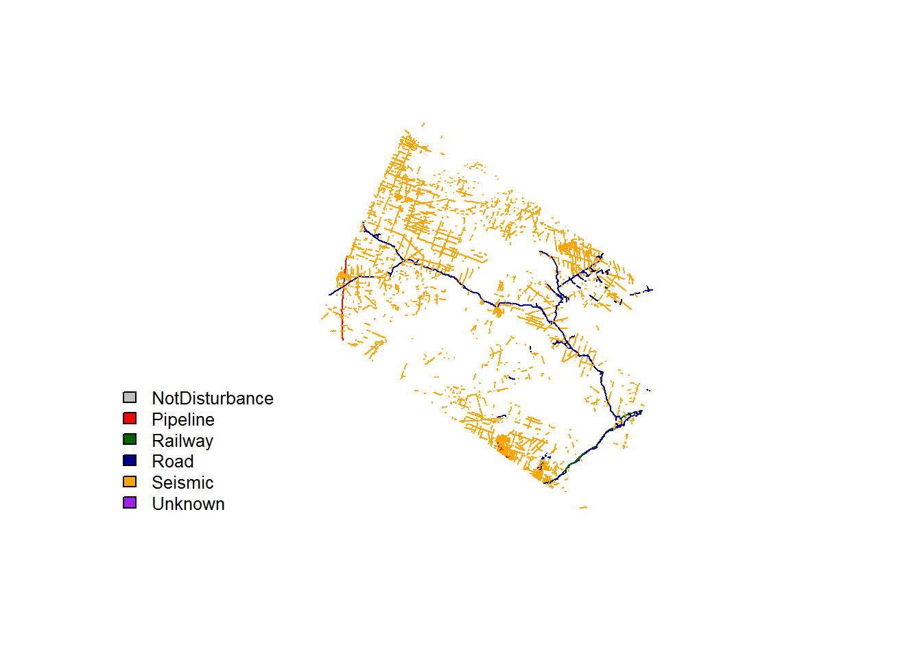
You can see mostly seismic lines and roads. Here they are on an interactive mapview imagery:
require(mapview)
mapview(BEAD.lines[,"Class"], map.types = "Esri.WorldImagery")1.1 Calculate density (km/km2) of linear features
This is the first somewhat tricky task. We’ll do this for a sample portion of the map first to speed up processing time. st_crop crops the shapefile to the listed extent:
require(raster)
BEAD.crop <- st_crop(BEAD.lines, extent(-1253023, -1227564, 2546649, 2578169))
plot(BEAD.crop[,"Class"])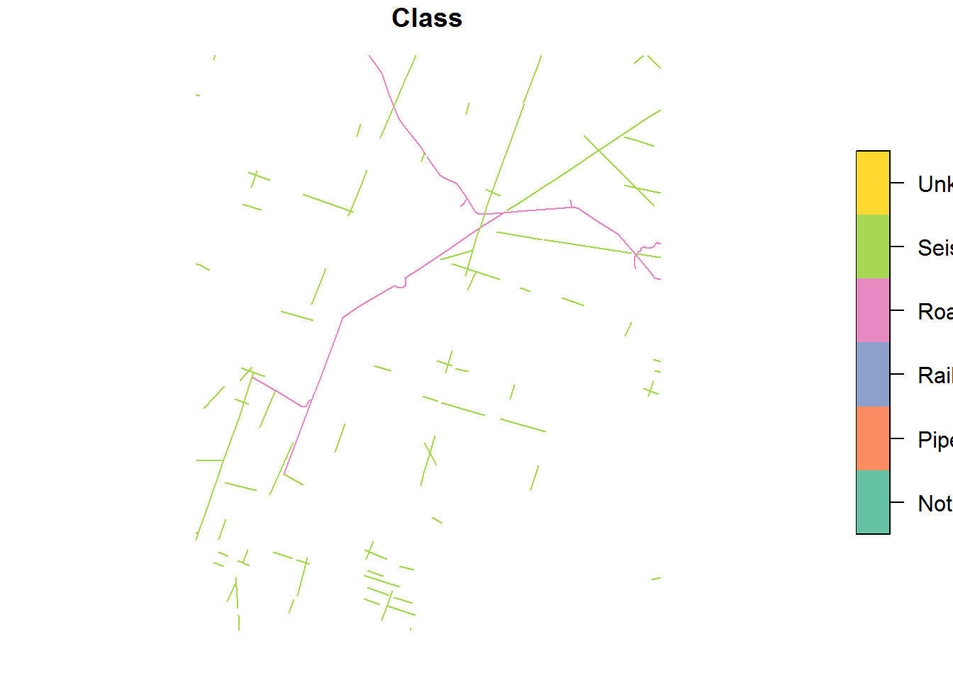
BEAD.crop.sp <- as(BEAD.crop, "Spatial")as(,"Spatial") converts an sf object to a spatial object. Alternatively, you can use as.Spatial().
We use a multi-step process to calculate the density of linear features:
- Make an empty raster with the same extent as the linear features shapefile
- Make a shapefile of the empty raster
- Cut the linear features at the transitions between pixels using the new shapefile
- Populate the empty raster with the sum of the lengths of the linear features that intersect it.
Steps 2 and 3 are important for the accuracy of the density calculation when using this method. The method used here measures the length of all linear features that intersect with a pixel and adds them together. That means if a road intersects with a pixel, it will measure the length of the entire road, not just the part within that pixel. Steps 2 and 3 cut the linear features at the borders between pixels, so that when you measure the lengths in step 4 you count only the portion of each linear feature that is inside that particular pixel.
require(plyr)
require(rgeos)First we make an empty raster. It should have the same extent and projection as the cropped shapefile:
empty.raster <- raster(extent(BEAD.crop), resolution = 3000, crs = projection(BEAD.crop))Next, make a shapefile from the empty raster that looks like a grid, i.e. the outline of each pixel. rasterToPolygons(raster package) makes a shapefile of the outline of each pixel.
density.poly <- rasterToPolygons(empty.raster)
plot(density.poly)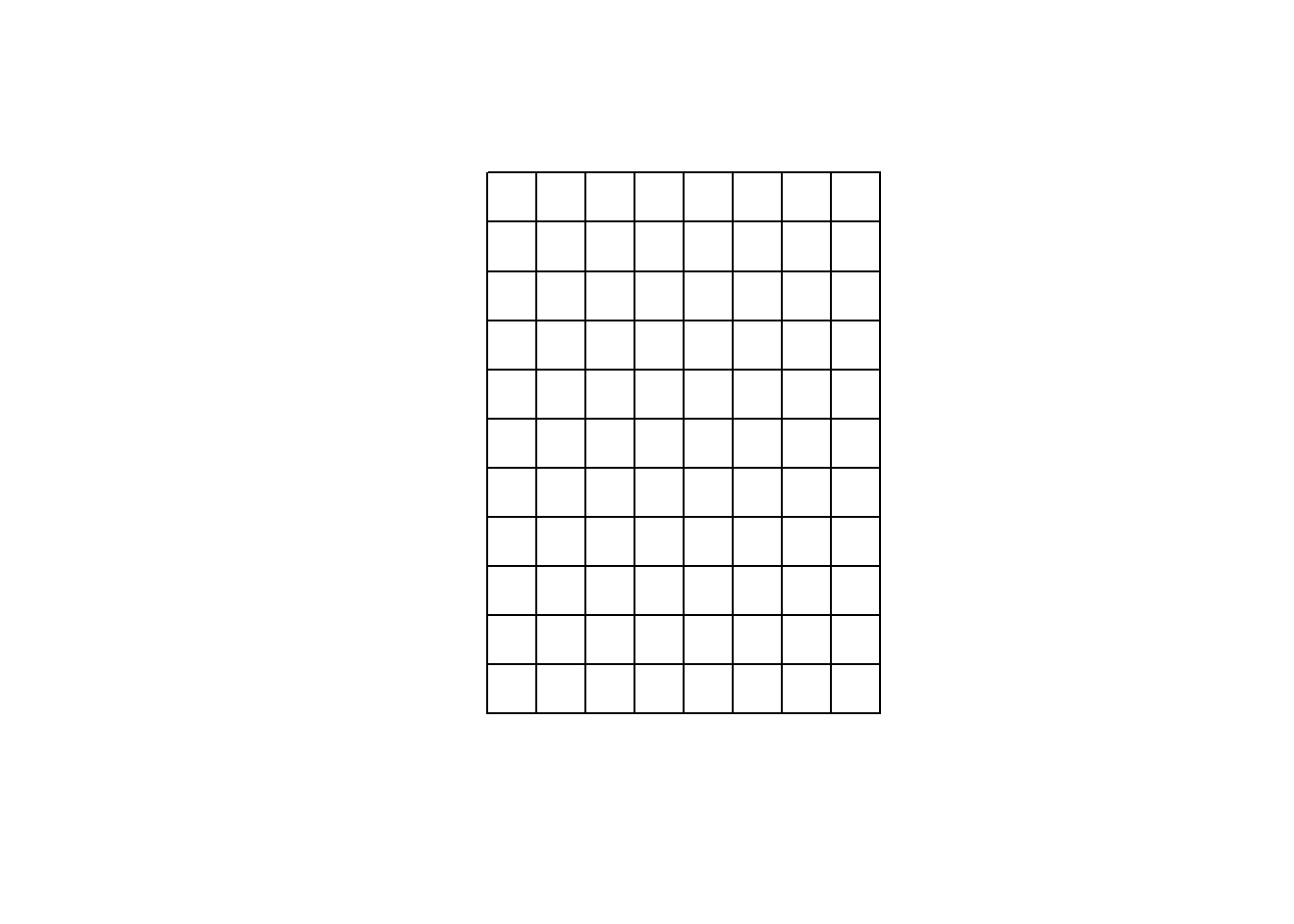
The tricky step is to “intersect” the lines with his grid, which cuts the linear features at the edges.gIntersection(rgeos package) is a function for determining the intersection between two given geometries (in this case, density.poly and BEAD.crop.sp). Note, the byid = TRUE in the gIntersection function makes sure that the clipping occurs for EACH polygon. The later stuff converts it back to a simple feature.
require(magrittr)
lines.clipped <- gIntersection(density.poly, BEAD.crop.sp, byid = TRUE) %>%
st_as_sf %>% mutate(length = st_length(geometry))We now have a simple feature with segments cut into the new raster with a computed “length” column:
lines.clipped## Simple feature collection with 173 features and 1 field
## geometry type: LINESTRING
## dimension: XY
## bbox: xmin: -1253023 ymin: 2546649 xmax: -1229023 ymax: 2578169
## epsg (SRID): NA
## proj4string: +proj=aea +lat_1=50 +lat_2=70 +lat_0=40 +lon_0=-96 +x_0=0 +y_0=0 +ellps=GRS80 +towgs84=0,0,0,0,0,0,0 +units=m +no_defs
## First 10 features:
## geometry length
## 1 LINESTRING (-1252069 257794... 235.85716 m
## 2 LINESTRING (-1253023 257602... 216.56771 m
## 3 LINESTRING (-1242183 257537... 222.31043 m
## 4 LINESTRING (-1243536 257816... 3130.52798 m
## 5 LINESTRING (-1243745 257816... 7.74042 m
## 6 LINESTRING (-1241023 257809... 2954.10981 m
## 7 LINESTRING (-1242183 257537... 219.81122 m
## 8 LINESTRING (-1240989 257816... 85.83307 m
## 9 LINESTRING (-1238037 257556... 412.51364 m
## 10 LINESTRING (-1235023 257568... 97.96807 mplot(density.poly, border = "grey")
plot(lines.clipped, add = TRUE, lwd = 2)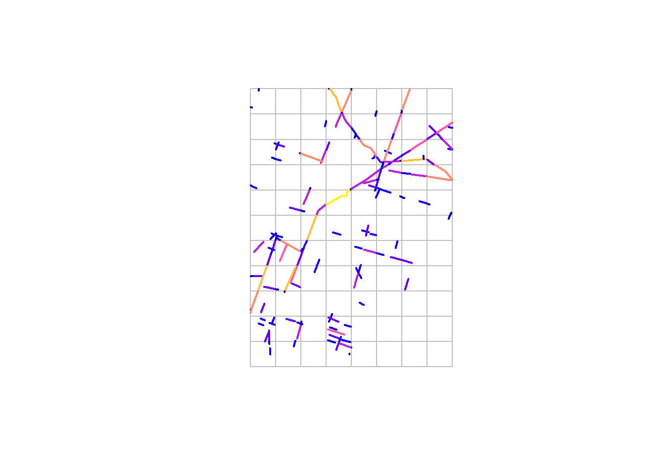
Finally, we populate the empty raster with the sum of the lengths of the linear features that intersect it using the rasterize command. The.
lines.clipped$length <- as.numeric(lines.clipped$length)/1e3
density.raster <- rasterize(as(lines.clipped, "Spatial"),
empty.raster,
field = "length", fun="sum")/9The rasterize is pretty slow Extra credit: Is there a way to do this very quickly with fasterize? I’m not sure!
Note - the first line converts the distance to km. The ./9 in the second line takes into account the fact that our raster is 3km x 3km, so to get to km/km^2 we divide by 9.
Plot the linear features over your new density raster
palette(topo.colors(100))
plot(density.raster/9)
plot(BEAD.crop[,"Class"], add = TRUE, lwd = 2, pal = rainbow)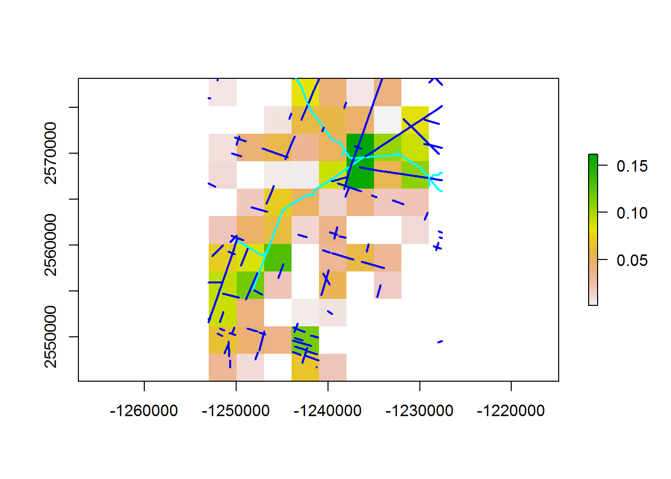
OR, you can use mapview for a nicer visualization against a map:
m1 <- mapview(density.raster, map.types = "Esri.WorldImagery")
mapview(BEAD.crop[,"Class"], map = m1@map)The mapview features are great for confirming that these spatial analyses are working, as you can zoom in to any particular pixel, and scroll over any particular line segment.
Some key functions used in this code:
rasterToPolygons- inrasterrasterize- inrasterst_length- insf- Several times we had to convert between “Spatial” and “simple feature” type objects using
st_as_sf(converts spatial to sf) andas(., "Spatial")- (sf to spatial).
1.1.1 All in one function
This function takes an sf of lines, a resolution (in m) of the desired raster, and a plotme flag - whether to plot it or not.
getLineDensity <- function(lines.sf, resolution, plotme = TRUE){
pcks <- c("plyr","rgeos","sp","sf","raster")
a <- sapply(pcks, require, character = TRUE)
empty.raster <- raster(extent(lines.sf),
resolution = resolution,
crs = projection(lines.sf))
density.poly <- rasterToPolygons(empty.raster)
lines.sp <- as(lines.sf, "Spatial")
lines.clipped <- gIntersection(density.poly, lines.sp, byid = TRUE) %>%
st_as_sf %>% mutate(length = st_length(geometry))
lines.clipped$length <- as.numeric(lines.clipped$length)/1e3
density.raster <- rasterize(as(lines.clipped, "Spatial"),
empty.raster, field = "length",
fun="sum")/((resolution/1e3)^2)
if(plotme){
plot(density.raster)
plot(st_geometry(lines.sf), add = TRUE, lwd = 2, pal = rainbow)
}
return(density.raster)
}Here, for exapmle, is the density raster for the same crop but at a finer (1km) resolution:
line.density1km <- getLineDensity(BEAD.crop, 1e3)
Or - for example - we can subset the roads and do the entire BEAD.lines domain at - say - a 10km resolution. The system.time() command is just to time this operation.
system.time(line.density10km <- getLineDensity(subset(BEAD.lines, Class == "Road"), 10e3))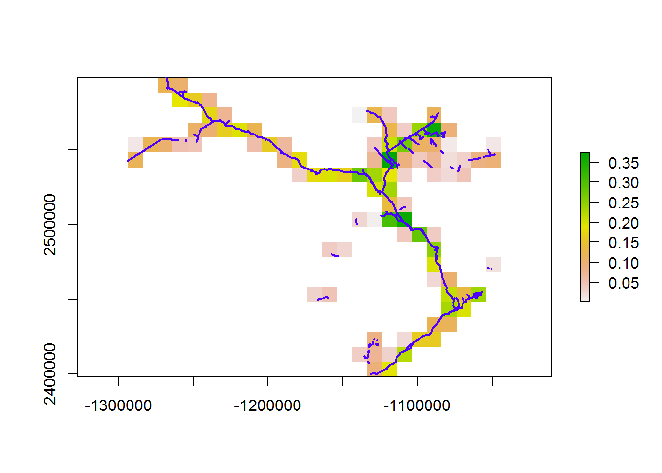
## user system elapsed
## 17.31 0.06 17.89Finally, the density of all linear elements at 10km resolution:
system.time(line.density10km <- getLineDensity(BEAD.lines, 10e3))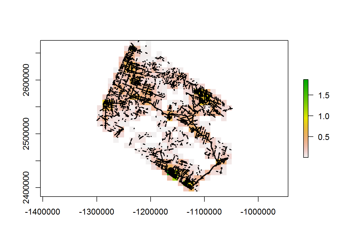
## user system elapsed
## 95.14 0.39 98.79And a little mapview imagery:
m1 <- mapview(line.density10km, map.types = "Esri.WorldImagery")
mapview(BEAD.lines[,"Class"], map = m1@map)1.2 Distance to linear elements
To obtain a raster of distances from nearest linear elements, we:
- find the centroids of the desired raster with
st_centroid - find the nearest distances between that set of centroids and the linear elements with
st_distance
Find centroids of the raster:
empty.raster <- raster(extent(BEAD.crop), resolution = 3000, crs = projection(BEAD.crop))
distance.poly <- rasterToPolygons(empty.raster)
distance.poly.sf <- st_as_sf(distance.poly)Now we can compute centroids:
distance.centroid <- st_centroid(distance.poly.sf)
plot(distance.poly)
plot(st_geometry(distance.centroid), add = TRUE)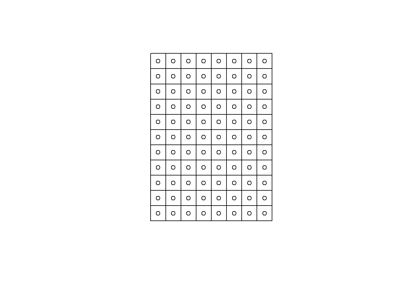
There is a slight hiccup before the next step: for some reason the conversion from spatial slightly changes the projection definition, which causes problems later …
st_crs(distance.centroid)## Coordinate Reference System:
## No EPSG code
## proj4string: "+proj=aea +lat_1=50 +lat_2=70 +lat_0=40 +lon_0=-96 +x_0=0 +y_0=0 +ellps=GRS80 +towgs84=0,0,0,0,0,0,0 +units=m +no_defs"st_crs(BEAD.crop)## Coordinate Reference System:
## No EPSG code
## proj4string: "+proj=aea +lat_1=50 +lat_2=70 +lat_0=40 +lon_0=-96 +x_0=0 +y_0=0 +datum=NAD83 +units=m +no_defs"distance.centroid <- st_transform(distance.centroid, st_crs(BEAD.crop))
st_crs(distance.centroid) == st_crs(BEAD.crop)## [1] TRUEObtain distances:
distances <- st_distance(distance.centroid, BEAD.crop)This generates a large matrix of all pairwise distances:
nrow(distance.centroid)## [1] 88nrow(BEAD.crop)## [1] 116dim(distances)## [1] 88 116We want the closest distance, which we obtain as:
distance.min <- apply(distances, 1, min)We can now populate the empty raster with these values:
distance.raster <- setValues(empty.raster, distance.min)Let’s check this:
plot(distance.raster)
plot(st_geometry(BEAD.crop), add = TRUE)
OR - with mapview:
m1 <- mapview(distance.raster, map.types = "Esri.WorldImagery")
mapview(BEAD.crop, m1@map)1.2.1 All in one function:
There are a few little tricks to this function to speed the processes up a bit (including a little cameo from our friend “fasterize”).
getDistanceToLines <- function(lines.sf, resolution, plotme = TRUE){
pcks <- c("plyr","rgeos","sp","sf","raster", "fasterize")
a <- sapply(pcks, require, character = TRUE)
xy <- st_coordinates(lines.sf)[,1:2]
mcp <- xy[chull(xy),] %>% rbind(xy[chull(xy)[1],]) %>% list %>% st_polygon %>% st_sfc %>% st_sf
empty.raster <- fasterize(mcp, raster(extent(lines.sf), resolution = resolution, crs = projection(lines.sf)))
# cut out portions of raster outside MCP
distance.centroid <- suppressWarnings(rasterToPolygons(empty.raster) %>% st_as_sf %>% st_centroid %>% st_transform(st_crs(lines.sf)))
distance.matrix <- st_distance(distance.centroid, lines.sf)
distance.min <- apply(distance.matrix, 1, min)
raster.vals <- getValues(empty.raster)
raster.vals[!is.na(raster.vals)] <- distance.min
distance.raster <- setValues(empty.raster, raster.vals)
if(plotme){
plot(distance.raster)
plot(st_geometry(lines.sf), add = TRUE)
}
return(distance.raster)
}Some examples as above:
- the distance raster for the same crop but at a finer (1km) resolution:
system.time(d.to.line_1km <- getDistanceToLines(BEAD.crop, 1e3))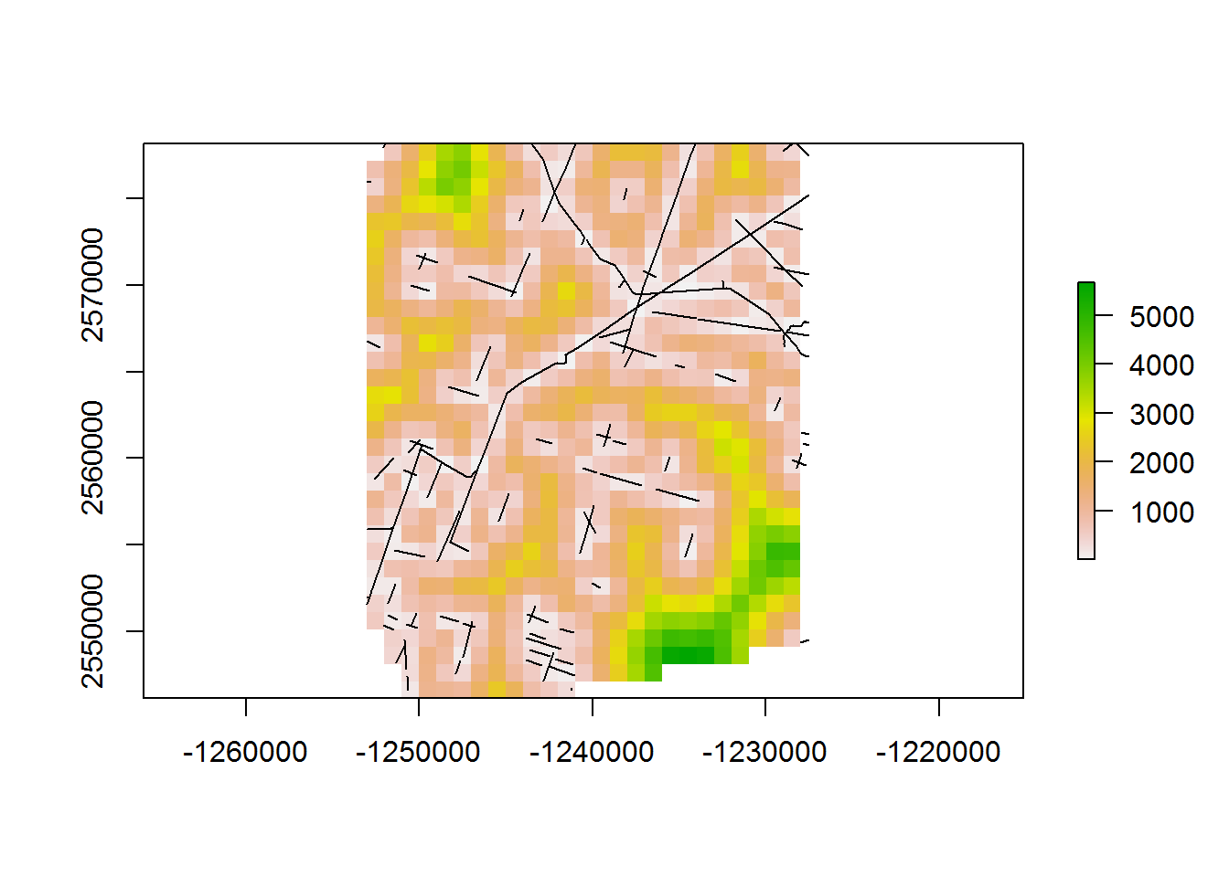
## user system elapsed
## 0.66 0.00 0.70- distance to roads, whole domain:
system.time(d.to.road_10km <- getDistanceToLines(subset(BEAD.lines, Class == "Road"), 10e3))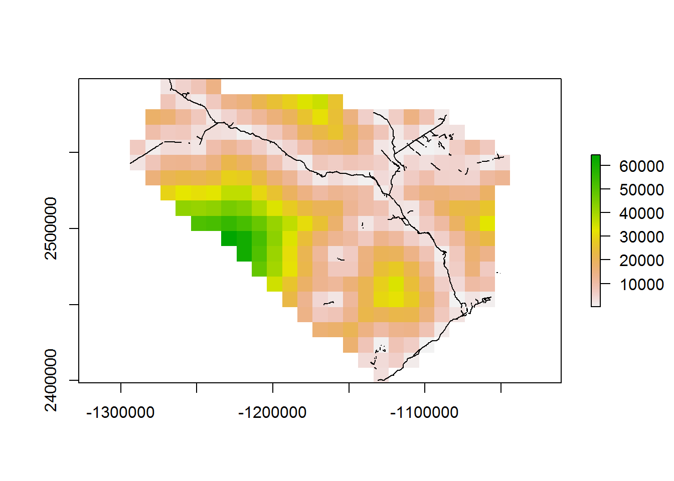
## user system elapsed
## 0.55 0.00 0.58This is fast enough that we can crank the resolution for all the lines down to 5 km no problem.
system.time(d.to.lines_10km <- getDistanceToLines(BEAD.lines, 5e3))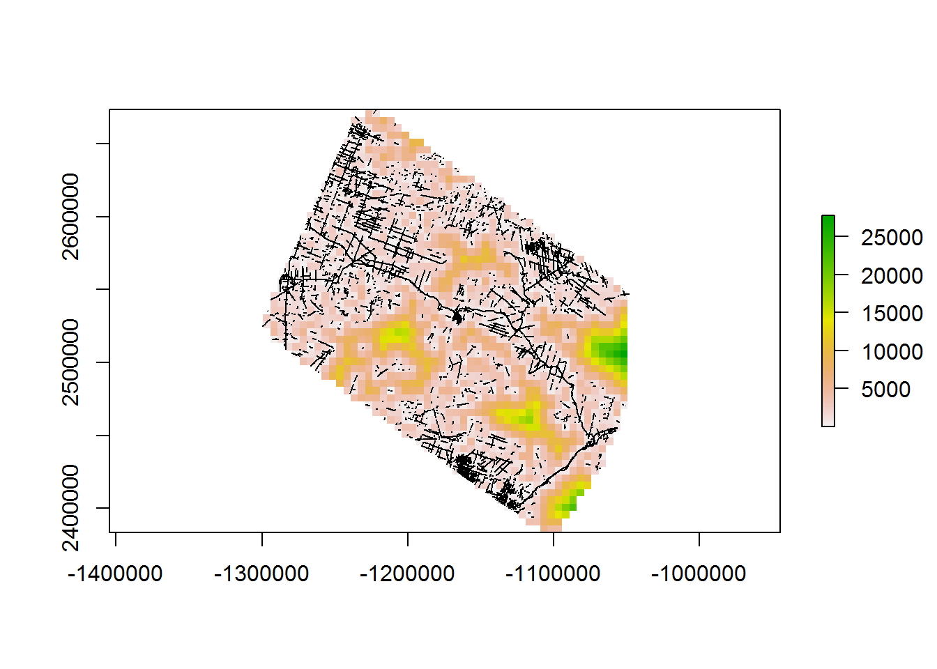
## user system elapsed
## 15.76 0.13 16.312 Polygons
The BEADpolys2015_NT1_Bistcho_Calendar_MaxH_Yates_HRL_clip.shp file contains the human disturbance polygon data:
require(sf)
BEAD.polys <- st_read("_data/BEAD/BEADpolys2015_NT1_Bistcho_Calendar_MaxH_Yates_HRL_clip.shp")## Reading layer `BEADpolys2015_NT1_Bistcho_Calendar_MaxH_Yates_HRL_clip' from data source `C:\Users\Guru\Box Sync\caribou\NWT\rsf\primers\_data\BEAD\BEADpolys2015_NT1_Bistcho_Calendar_MaxH_Yates_HRL_clip.shp' using driver `ESRI Shapefile'
## Simple feature collection with 294 features and 31 fields
## geometry type: POLYGON
## dimension: XY
## bbox: xmin: -1282731 ymin: 2399357 xmax: -1060151 ymax: 2620039
## epsg (SRID): NA
## proj4string: +proj=aea +lat_1=50 +lat_2=70 +lat_0=40 +lon_0=-96 +x_0=0 +y_0=0 +datum=NAD83 +units=m +no_defsA plot of the data:
require(scales)
colors <- c("grey", "red", "darkgreen", "darkblue", "orange", "purple")
plot(st_geometry(BEAD.polys), col = colors[BEAD.polys$Class], main = "BEADpolys")
legend("bottomleft", fill = colors, legend = levels(BEAD.polys$Class), bty = "n", cex = 0.8)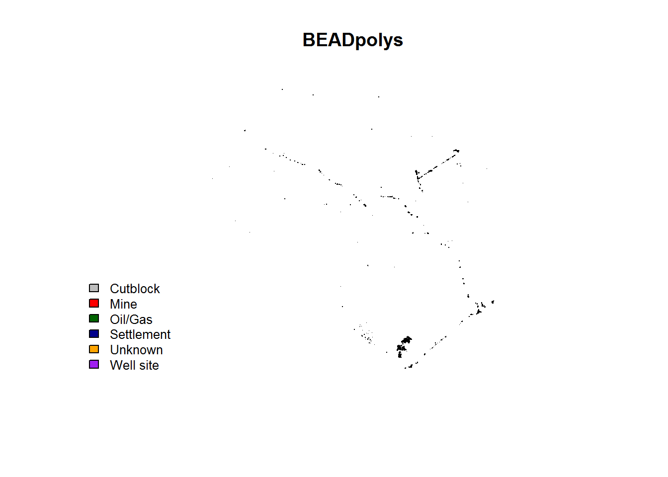
A table of class types:
BEAD.polys$Class %>% table## .
## Cutblock Mine Oil/Gas Settlement Unknown Well site
## 62 8 3 43 15 163They are widely and sparsely distributed, and (unsurprisingly) mainly along the roads.
Here’s a crop of the polygon file:
require(raster)
BEAD.polys.crop <- st_crop(BEAD.polys, extent(-1147153, -1119731, 2405299, 2427824))
plot(BEAD.polys.crop[,"Class"])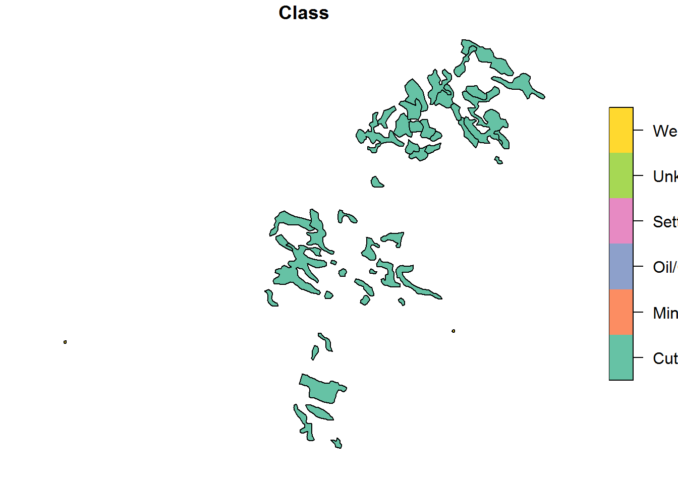
It is illuminating to see where these polygons line up against ESRI world imagery (its not that great!)
mapview(BEAD.polys.crop[,"Class"], map.types = "Esri.WorldImagery")Our goal will be to find densities of polygons and nearest distances to polygons, as for the linear elements above.
In this crop, there are 48 features, of which almost all at “Cutblocks”:
table(BEAD.polys.crop$Class)##
## Cutblock Mine Oil/Gas Settlement Unknown Well site
## 46 0 0 0 0 22.1 Calculate density of polygonal features
We will take the polygon data and compute the density into a 1km raster. In the code below, there are 5 steps:
- Create an empty 1x1 km raster:
empty.raster <- raster(extent(BEAD.polys.crop), resolution = 1e3, crs = projection(BEAD.polys.crop))- Convert to a polygon data type. Note that
rasterToPolygonsmakes aSpatialdata object, NOT asimple feature… this is another function that some time soon (if not already) will be doable withsf:
polys.grid.st <- rasterToPolygons(empty.raster) - Obtain the interection between the two poygon data sets. Note, we have to convert the BEAD polygon to
Spatialas well. Note also, that thebyid = TRUEis necessary to get the very specific slicing of the two polygon data sets:
require(rgeos)
polys.raster.intersection <- gIntersection(polys.grid.st, as(BEAD.polys.crop, "Spatial"), byid = TRUE)
plot(polys.raster.intersection)
- Importantlty, we need to extract the index of the appropriate raster polygon, to correctly populate the raster. Note that the names of the ensuing intersected polygons combine the indices of each of the polygons in the original dataset:
head(names(polys.raster.intersection))## [1] "17 60" "17 182" "18 182" "19 182" "34 185" "35 61"We need the first number in each pair. The following bit of code is one way to do that:
index <- sapply(strsplit(names(polys.raster.intersection), " "), head, 1) %>% as.numeric - Extract the area of each of the polygons. I find this is easier switching back to simple features:
areas <- st_area(st_as_sf(polys.raster.intersection))- Populate the raster - but carefully, because several of the polygons have multiple area values to fill. So first, we need to compute the total area in each raster block:
area.final <- tapply(areas, index, sum)
index.final <- unique(index)Now we know exactly where to place these.
empty.raster[index.final] <- area.final/1e6
plot(empty.raster)
plot(BEAD.polys.crop, add = TRUE)
2.2 In a single function
All together as a function. Note that I added an “overlapping” tag. If the polygons are NOT overlapping, the function is much faster because it can “collapse” all of the polygons into a single object with the gUnaryUnion function:
getPolygonDensity <- function(polys.sf, resolution, plotme = TRUE, overlapping = FALSE){
pcks <- c("plyr","rgeos","sp","sf","raster","fasterize")
a <- sapply(pcks, require, character = TRUE)
density.raster <- raster(extent(polys.sf),
resolution = resolution,
crs = projection(polys.sf))
raster.poly <- rasterToPolygons(density.raster)
polys.sp <- as(polys.sf, "Spatial")
if(!overlapping) polys.sp <- gUnaryUnion(polys.sp)
polys.raster.intersection <- gIntersection(raster.poly, polys.sp, byid = TRUE)
pri.sf <- st_as_sf(polys.raster.intersection)
pri.sf$area <- st_area(pri.sf)
index <- sapply(strsplit(names(polys.raster.intersection), " "), head, 1) %>% as.numeric
areas <- st_area(st_as_sf(polys.raster.intersection))
area.final <- tapply(areas, index, sum)
index.final <- unique(index)
density.raster[index.final] <- area.final/1e6
if(plotme){
plot(density.raster)
plot(st_geometry(polys.sf), add = TRUE)
}
return(density.raster)
}Some examples - at 1km:
system.time(getPolygonDensity(BEAD.polys.crop, 1000))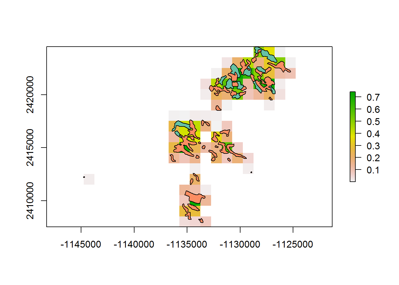
## user system elapsed
## 0.40 0.00 0.45At 0.5 km:
system.time(getPolygonDensity(BEAD.polys.crop, 500))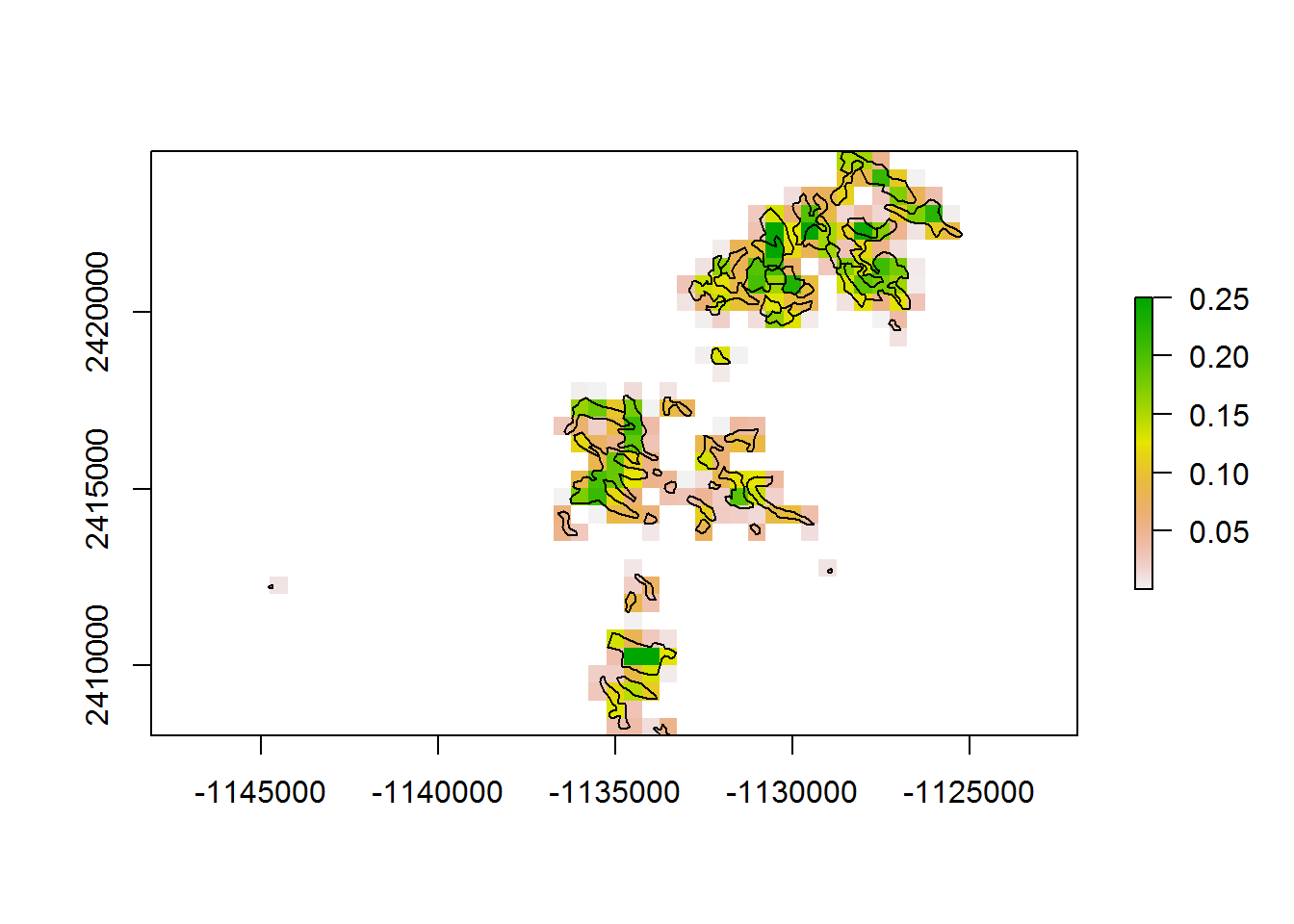
## user system elapsed
## 0.98 0.02 1.00At 5 km for entire range, comparing overlapping and non-overlapping:
system.time(a <- getPolygonDensity(BEAD.polys, 5000, overlapping = TRUE))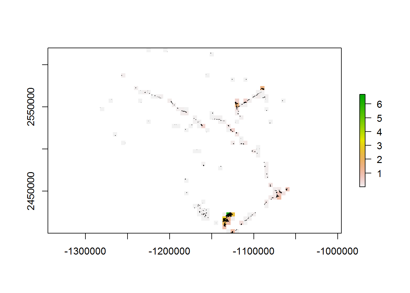
## user system elapsed
## 8.66 0.05 8.92system.time(b <- getPolygonDensity(BEAD.polys, 5000, overlapping = FALSE))
## user system elapsed
## 5.02 0.04 5.153 Complete code
Click below to show complete code from this document.
knitr::opts_chunk$set(echo = TRUE, cache=TRUE, message = FALSE, warning = FALSE)
require(sf)
BEAD.lines <- st_read("_data/BEAD/BEADlines2015_NT1_Bistcho_Calendar_MaxH_Yates_HRL_clip.shp")
head(BEAD.lines)
require(scales)
colors <- c("grey", "red", "darkgreen", "darkblue", "orange", "purple")
plot(st_geometry(BEAD.lines), col = colors[BEAD.lines$Class])
legend("bottomleft", fill = colors, legend = levels(BEAD.lines$Class), bty = "n", cex = 0.8)
require(mapview)
mapview(BEAD.lines[,"Class"], map.types = "Esri.WorldImagery")
require(raster)
BEAD.crop <- st_crop(BEAD.lines, extent(-1253023, -1227564, 2546649, 2578169))
plot(BEAD.crop[,"Class"])
BEAD.crop.sp <- as(BEAD.crop, "Spatial")
require(plyr)
require(rgeos)
empty.raster <- raster(extent(BEAD.crop), resolution = 3000, crs = projection(BEAD.crop))
density.poly <- rasterToPolygons(empty.raster)
plot(density.poly)
require(magrittr)
lines.clipped <- gIntersection(density.poly, BEAD.crop.sp, byid = TRUE) %>%
st_as_sf %>% mutate(length = st_length(geometry))
lines.clipped
plot(density.poly, border = "grey")
plot(lines.clipped, add = TRUE, lwd = 2)
lines.clipped$length <- as.numeric(lines.clipped$length)/1e3
density.raster <- rasterize(as(lines.clipped, "Spatial"),
empty.raster,
field = "length", fun="sum")/9
palette(topo.colors(100))
plot(density.raster/9)
plot(BEAD.crop[,"Class"], add = TRUE, lwd = 2, pal = rainbow)
require(mapview)
m1 <- mapview(density.raster, map.types = "Esri.WorldImagery")
mapview(BEAD.crop[,"Class"], map = m1@map)
getLineDensity <- function(lines.sf, resolution, plotme = TRUE){
pcks <- c("plyr","rgeos","sp","sf","raster")
a <- sapply(pcks, require, character = TRUE)
empty.raster <- raster(extent(lines.sf),
resolution = resolution,
crs = projection(lines.sf))
density.poly <- rasterToPolygons(empty.raster)
lines.sp <- as(lines.sf, "Spatial")
lines.clipped <- gIntersection(density.poly, lines.sp, byid = TRUE) %>%
st_as_sf %>% mutate(length = st_length(geometry))
lines.clipped$length <- as.numeric(lines.clipped$length)/1e3
density.raster <- rasterize(as(lines.clipped, "Spatial"),
empty.raster, field = "length",
fun="sum")/((resolution/1e3)^2)
if(plotme){
plot(density.raster)
plot(st_geometry(lines.sf), add = TRUE, lwd = 2, pal = rainbow)
}
return(density.raster)
}
line.density1km <- getLineDensity(BEAD.crop, 1e3)
system.time(line.density10km <- getLineDensity(subset(BEAD.lines, Class == "Road"), 10e3))
system.time(line.density10km <- getLineDensity(BEAD.lines, 10e3))
require(mapview)
m1 <- mapview(line.density10km, map.types = "Esri.WorldImagery")
mapview(BEAD.lines[,"Class"], map = m1@map)
empty.raster <- raster(extent(BEAD.crop), resolution = 3000, crs = projection(BEAD.crop))
distance.poly <- rasterToPolygons(empty.raster)
distance.poly.sf <- st_as_sf(distance.poly)
distance.centroid <- st_centroid(distance.poly.sf)
plot(distance.poly)
plot(st_geometry(distance.centroid), add = TRUE)
st_crs(distance.centroid)
st_crs(BEAD.crop)
distance.centroid <- st_transform(distance.centroid, st_crs(BEAD.crop))
st_crs(distance.centroid) == st_crs(BEAD.crop)
distances <- st_distance(distance.centroid, BEAD.crop)
nrow(distance.centroid)
nrow(BEAD.crop)
dim(distances)
distance.min <- apply(distances, 1, min)
distance.raster <- setValues(empty.raster, distance.min)
plot(distance.raster)
plot(st_geometry(BEAD.crop), add = TRUE)
require(mapview)
m1 <- mapview(distance.raster, map.types = "Esri.WorldImagery")
mapview(BEAD.crop, m1@map)
getDistanceToLines <- function(lines.sf, resolution, plotme = TRUE){
pcks <- c("plyr","rgeos","sp","sf","raster", "fasterize")
a <- sapply(pcks, require, character = TRUE)
xy <- st_coordinates(lines.sf)[,1:2]
mcp <- xy[chull(xy),] %>% rbind(xy[chull(xy)[1],]) %>% list %>% st_polygon %>% st_sfc %>% st_sf
empty.raster <- fasterize(mcp, raster(extent(lines.sf), resolution = resolution, crs = projection(lines.sf)))
# cut out portions of raster outside MCP
distance.centroid <- suppressWarnings(rasterToPolygons(empty.raster) %>% st_as_sf %>% st_centroid %>% st_transform(st_crs(lines.sf)))
distance.matrix <- st_distance(distance.centroid, lines.sf)
distance.min <- apply(distance.matrix, 1, min)
raster.vals <- getValues(empty.raster)
raster.vals[!is.na(raster.vals)] <- distance.min
distance.raster <- setValues(empty.raster, raster.vals)
if(plotme){
plot(distance.raster)
plot(st_geometry(lines.sf), add = TRUE)
}
return(distance.raster)
}
system.time(d.to.line_1km <- getDistanceToLines(BEAD.crop, 1e3))
system.time(d.to.road_10km <- getDistanceToLines(subset(BEAD.lines, Class == "Road"), 10e3))
system.time(d.to.lines_10km <- getDistanceToLines(BEAD.lines, 5e3))
require(sf)
BEAD.polys <- st_read("_data/BEAD/BEADpolys2015_NT1_Bistcho_Calendar_MaxH_Yates_HRL_clip.shp")
require(scales)
colors <- c("grey", "red", "darkgreen", "darkblue", "orange", "purple")
plot(st_geometry(BEAD.polys), col = colors[BEAD.polys$Class], main = "BEADpolys")
legend("bottomleft", fill = colors, legend = levels(BEAD.polys$Class), bty = "n", cex = 0.8)
BEAD.polys$Class %>% table
require(raster)
BEAD.polys.crop <- st_crop(BEAD.polys, extent(-1147153, -1119731, 2405299, 2427824))
plot(BEAD.polys.crop[,"Class"])
require(mapview)
mapview(BEAD.polys.crop[,"Class"], map.types = "Esri.WorldImagery")
table(BEAD.polys.crop$Class)
empty.raster <- raster(extent(BEAD.polys.crop), resolution = 1e3, crs = projection(BEAD.polys.crop))
polys.grid.st <- rasterToPolygons(empty.raster)
require(rgeos)
polys.raster.intersection <- gIntersection(polys.grid.st, as(BEAD.polys.crop, "Spatial"), byid = TRUE)
plot(polys.raster.intersection)
head(names(polys.raster.intersection))
index <- sapply(strsplit(names(polys.raster.intersection), " "), head, 1) %>% as.numeric
areas <- st_area(st_as_sf(polys.raster.intersection))
area.final <- tapply(areas, index, sum)
index.final <- unique(index)
empty.raster[index.final] <- area.final/1e6
plot(empty.raster)
plot(BEAD.polys.crop, add = TRUE)
getPolygonDensity <- function(polys.sf, resolution, plotme = TRUE, overlapping = FALSE){
pcks <- c("plyr","rgeos","sp","sf","raster","fasterize")
a <- sapply(pcks, require, character = TRUE)
density.raster <- raster(extent(polys.sf),
resolution = resolution,
crs = projection(polys.sf))
raster.poly <- rasterToPolygons(density.raster)
polys.sp <- as(polys.sf, "Spatial")
if(!overlapping) polys.sp <- gUnaryUnion(polys.sp)
polys.raster.intersection <- gIntersection(raster.poly, polys.sp, byid = TRUE)
pri.sf <- st_as_sf(polys.raster.intersection)
pri.sf$area <- st_area(pri.sf)
index <- sapply(strsplit(names(polys.raster.intersection), " "), head, 1) %>% as.numeric
areas <- st_area(st_as_sf(polys.raster.intersection))
area.final <- tapply(areas, index, sum)
index.final <- unique(index)
density.raster[index.final] <- area.final/1e6
if(plotme){
plot(density.raster)
plot(st_geometry(polys.sf), add = TRUE)
}
return(density.raster)
}
system.time(getPolygonDensity(BEAD.polys.crop, 1000))
system.time(getPolygonDensity(BEAD.polys.crop, 500))
system.time(a <- getPolygonDensity(BEAD.polys, 5000, overlapping = TRUE))
system.time(b <- getPolygonDensity(BEAD.polys, 5000, overlapping = FALSE))