Anthropogenic Disturbance: Line Density
Elie Gurarie
2019-09-27
1 The Goal:
We want to compute the density of linear elements (lines - in this case) with a radius \(r\) of any location in the figure. This is what ESRI/ArcGIS refers to as the Line Density Tool. Here’s a figure of their schematic:
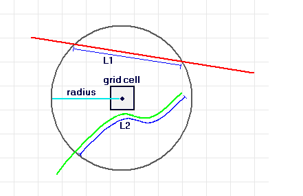
image
2 Data
Loading some linear element data, and getting a manageable crop (as in the previous primer).
require(sf)
require(raster)
BEAD.lines <- st_read("_data/BEAD/BEADlines2015_NT1_Bistcho_Calendar_MaxH_Yates_HRL_clip.shp")
## Reading layer `BEADlines2015_NT1_Bistcho_Calendar_MaxH_Yates_HRL_clip' from data source `C:\Users\Elie\Box Sync\caribou\NWT\rsf\primers\_data\BEAD\BEADlines2015_NT1_Bistcho_Calendar_MaxH_Yates_HRL_clip.shp' using driver `ESRI Shapefile'
## Simple feature collection with 4063 features and 32 fields
## geometry type: MULTILINESTRING
## dimension: XY
## bbox: xmin: -1299584 ymin: 2381243 xmax: -1048374 ymax: 2673503
## epsg (SRID): NA
## proj4string: +proj=aea +lat_1=50 +lat_2=70 +lat_0=40 +lon_0=-96 +x_0=0 +y_0=0 +datum=NAD83 +units=m +no_defsBEAD.crop <- st_crop(BEAD.lines, extent(-1253e3, -1228e3, 2547e3, 2578e3))
plot(BEAD.crop[,"Class"])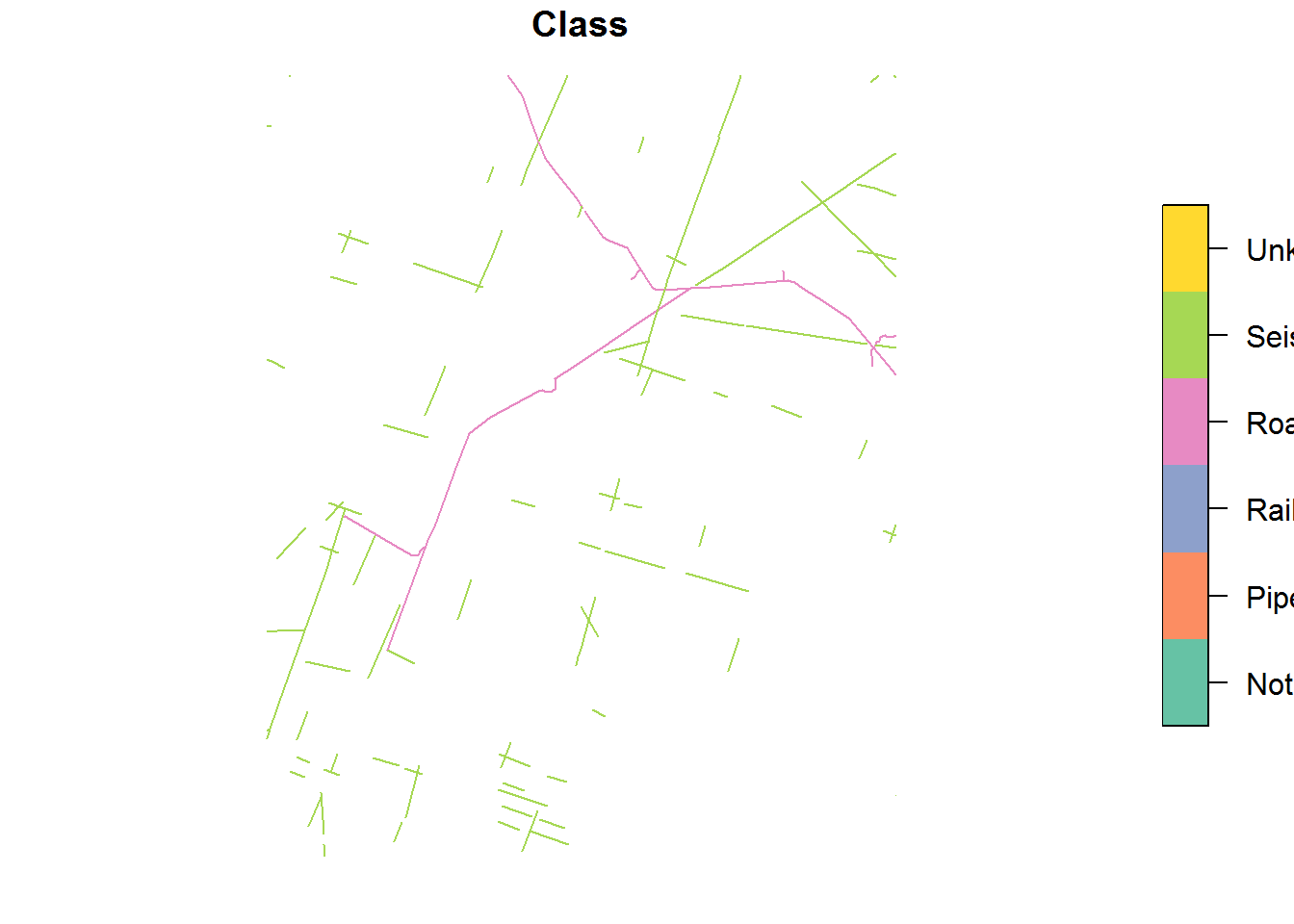
3 getLineDensity function
The following function computes the line density at point pt from a set of lines at radius r
getLineDensity <- function(pt, lines, r, plotme = FALSE){
pt.circle <- st_buffer(pt, r)
intersect <- st_intersection(pt.circle, lines)
length <- sum(st_length(intersect))/1e3 # in km
density <- (as.numeric(length)/(pi*(r/1e3)^2)) # in km/km^2
if(plotme){
plot(st_geometry(lines))
plot(pt.circle, add = TRUE, border = 2)
plot(intersect, add = TRUE, col =3)
}
return(density)
}The key functions here are (a) st_buffer, which draws a circular buffer around a point, (b) st_intersect, which intersects the lines through that buffer, and (c) st_length, which calculates the length of that intersection. The plotme toggle is just there so you can visualize the intersection.
For example, here is a point somewhere in the middle of the figure (note, for all the advantages of simple features, just creating a points is ugly!):
point <- st_point(c(-1240e3, 2560e3), dim = "XY") %>% st_sfc %>% st_sf(crs = st_crs(BEAD.crop))
getLineDensity(point, BEAD.crop, r = 5e3, plotme = TRUE)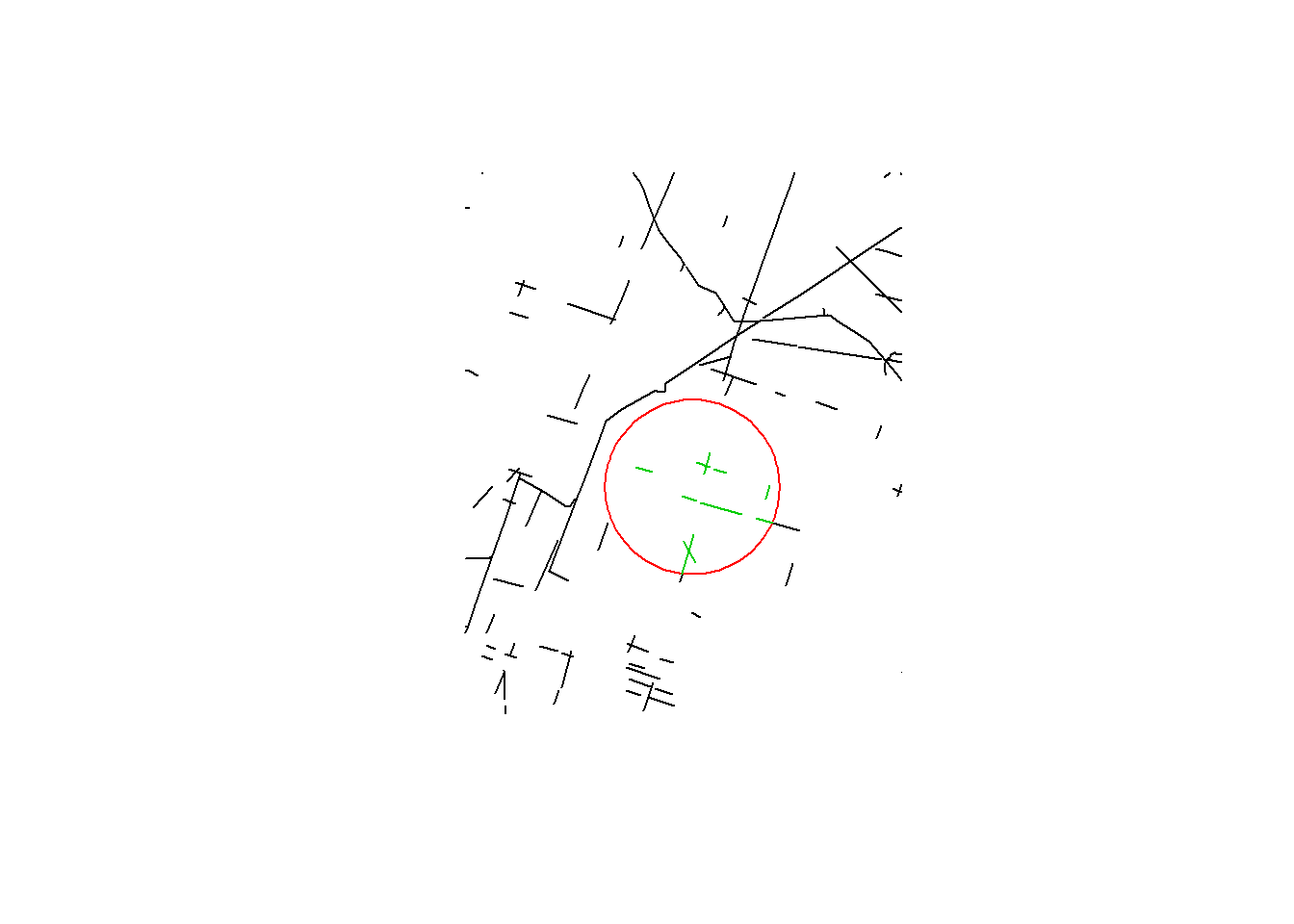
## [1] 0.1615591The value tells us, in km/km^2, what the density of linear elements within a 5km radius is about 0.16. For a larger radius (that captures most of the area):
getLineDensity(point, BEAD.crop, r = 15e3, plotme = TRUE)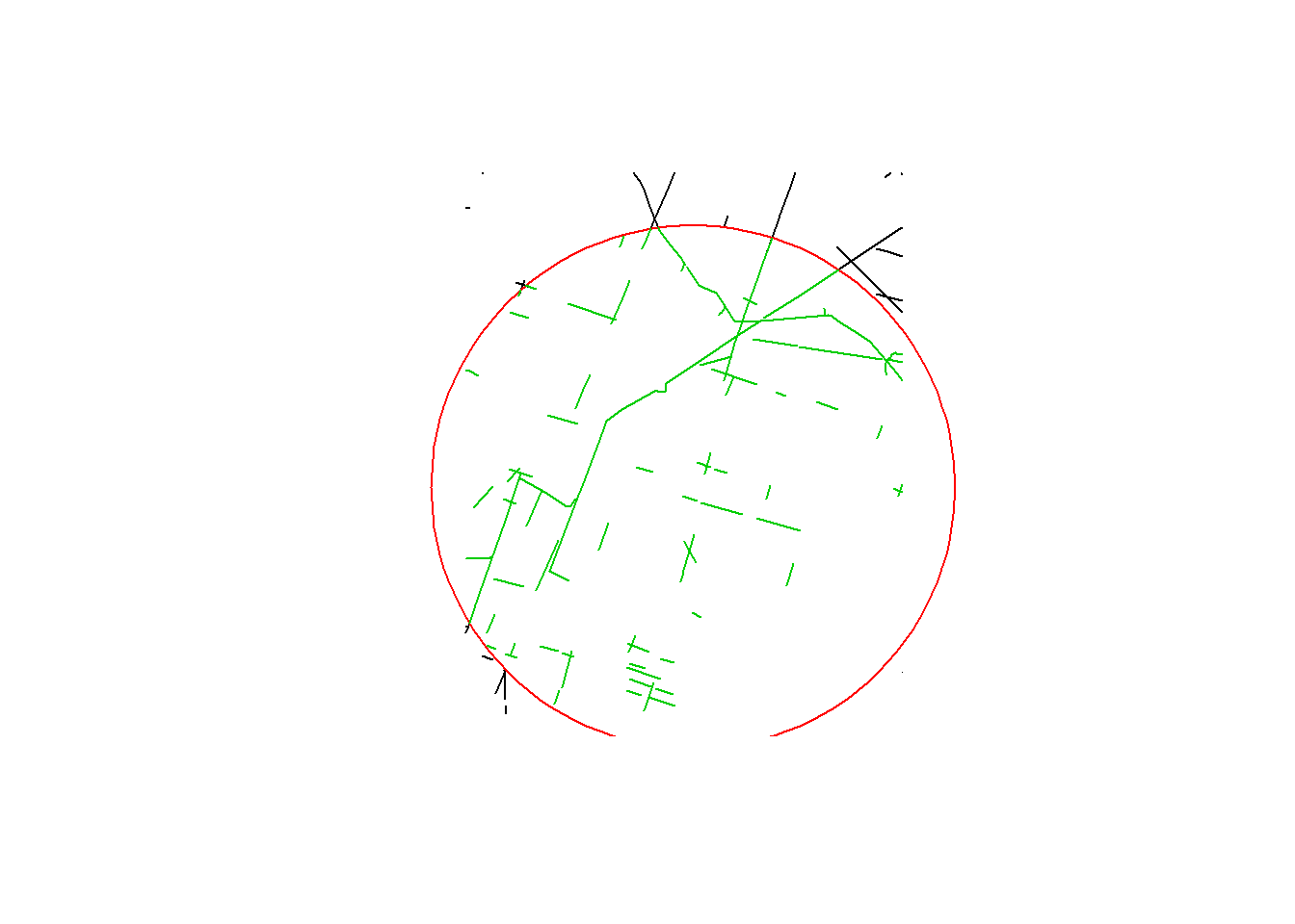
## [1] 0.2194583Note, you can easily break this down into the various components, e.g. road density:
getLineDensity(point, subset(BEAD.crop, Class == "Road"), r = 15e3, plotme = FALSE)## [1] 0.06358726vs. seismic line density
getLineDensity(point, subset(BEAD.crop, Class == "Seismic"), r = 15e3, plotme = FALSE)## [1] 0.1558713.1 Filling a raster
What we’d like to do is fill a raster with these values for each point. We follow the basic outline of the previous primer. We (1) create an empty raster, (2) obtains points for the center of every point in the raster, (3) compute the line densities at each of those points, and (4) fill the empty raster.
Here we do this in a loop, and time it. Note the dimensions of the raster is 62x50 (with a 500m resolution), i.e. 3100 cells:
density.raster <- raster(extent(BEAD.crop), resolution = 500, crs = st_crs(BEAD.crop))
density.poly <- rasterToPolygons(density.raster)
density.poly.sf <- st_as_sf(density.poly)
st_crs(density.poly.sf) <- st_crs(BEAD.crop)
densities <- rep(NA, nrow(density.poly.sf))
system.time(
for(i in 1:length(densities))
densities[i] <- getLineDensity(density.poly.sf[i,], lines = BEAD.crop, r = 1e3, plotme = FALSE)
)## user system elapsed
## 42.09 0.10 42.26values(density.raster) <- densities
plot(density.raster)
This is pretty slow (nearly a minute on a decent desktop), considering that the resolution of thies raster is not THAT low. There are a few ways to speed this up …
3.1.1 Speed up #1: apply functions
The R apply family of functions can often be faster than looping. Here’s an example where we use the split function to break the raster points into a list, and then use sapply to go down the whole list. Why is this faster? I’m not sure (apply functions aren’t supposed to be necessarily faster than loops), but …
density.poly.list <- split(density.poly.sf, 1:nrow(density.poly.sf))
system.time(
densities <- sapply(density.poly.list, getLineDensity, lines = BEAD.crop, r = 1e3)
)## user system elapsed
## 45.04 0.00 45.15values(density.raster) <- densities
plot(density.raster)
it is faster by about 10% (on my computer).
3.1.2 Speed up #2: Buffering lines
Plenty of points in the raster are outside of the 1km radius, and we shouldn’t even bother to calculate those. The following code excludes those points:
r <- 1e3
BEAD.crop.buffered <- st_buffer(BEAD.crop, r) %>% st_union
plot(st_geometry(BEAD.crop.buffered))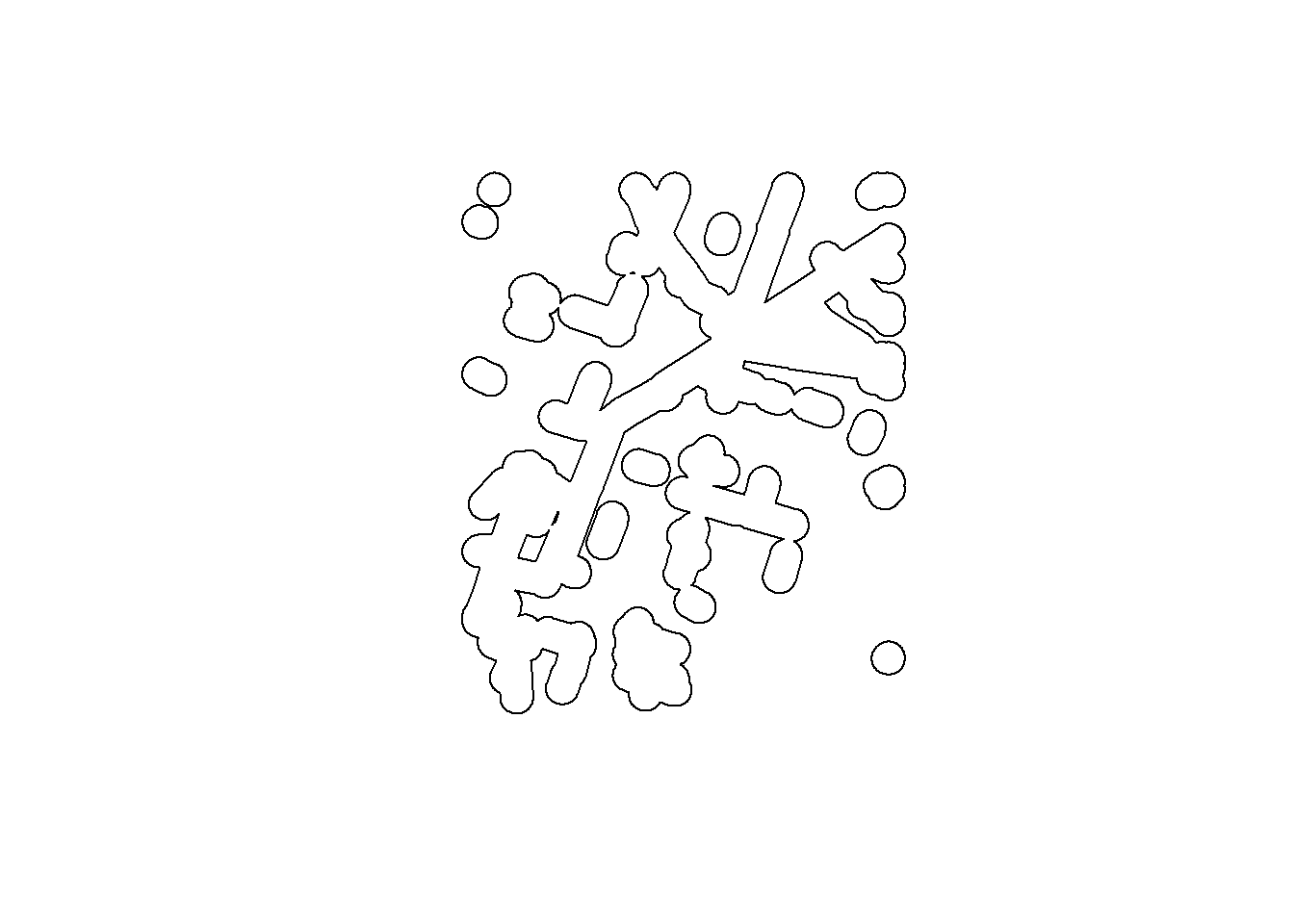
We can use this to preemptively only compute the density values within that buffer. This time we only loop through the indices in which.in.buffer:
which.in.buffer <- st_intersection(st_transform(density.poly.sf, st_crs(BEAD.crop.buffered)), st_geometry(BEAD.crop.buffered)) %>% row.names %>% as.numeric
densities <- rep(0, nrow(density.poly.sf))
density.poly.list <- split(density.poly.sf[which.in.buffer,], 1:length(which.in.buffer))
system.time(
densities.in.buffer <- sapply(density.poly.list, getLineDensity, lines = BEAD.crop, r = 1e3)
)## user system elapsed
## 27.37 0.05 27.41values(density.raster)[which.in.buffer] <- densities.in.buffer
plot(density.raster)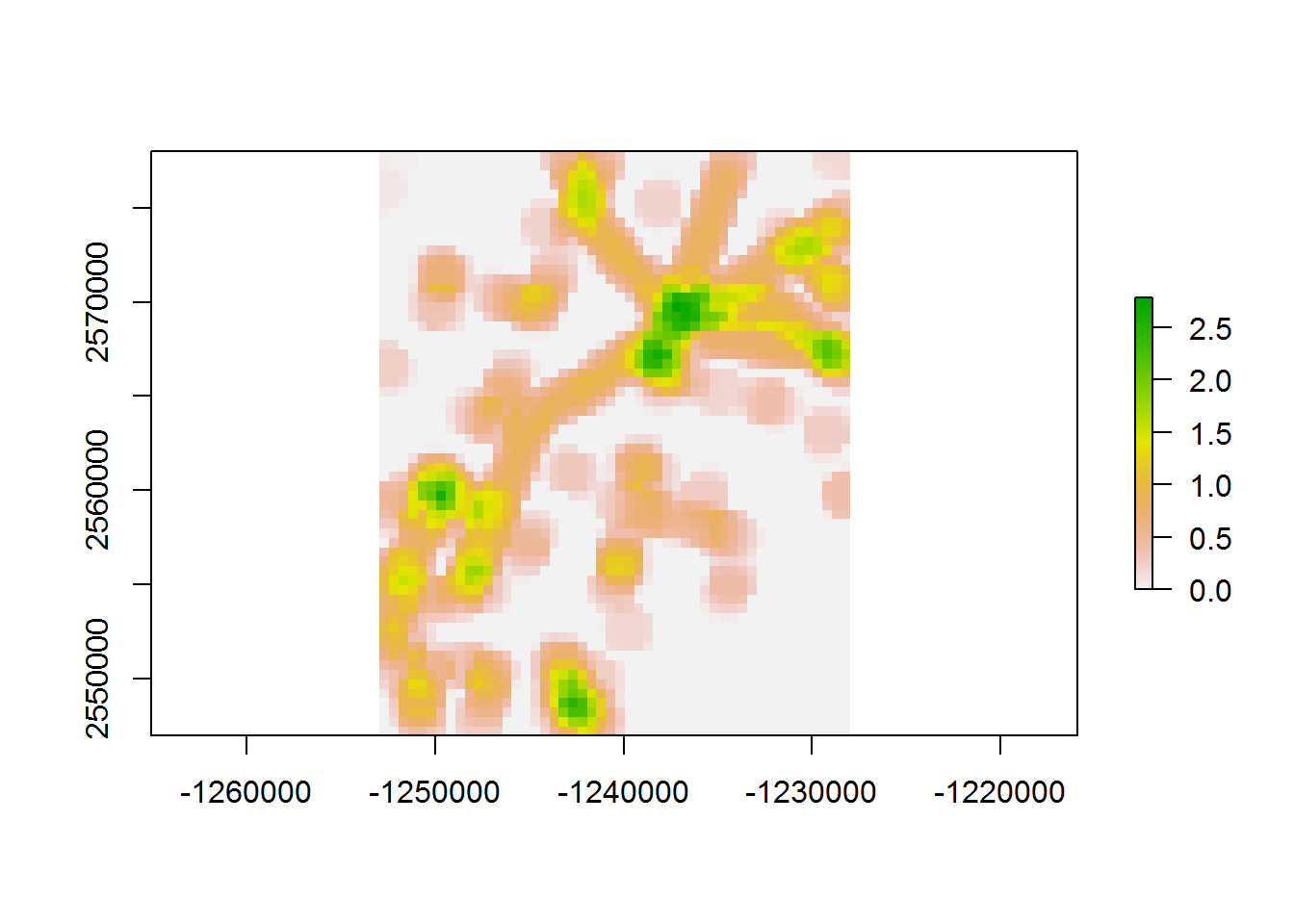
That cut computation time by nearly a factor of 3 compared to our first loop. A big improvement!
3.1.3 Speed up #3: Parallelization!
Once you’ve reduced a computation to its bare essentials, the next best way to speed up a computation is by parallelizing code, i.e. letting the multiple, usually idle, cores in your computer do some work for you. We are doing a simple loop here, so there is no reason that we can’t split this job up among several processors. There are plenty of resources on-line on parallel processing in R (e.g. here, here and here), and several packages that are helpful. There might be some differences between Windows and OS-X or Linus machines, but the basic ideas are similar. Below, I perform this process on my Windows laptop.
Here I will go through the workflow of performing the operation above using the doParallel package. First, the package(s):
require(doParallel)Determine the number of cores:
n <- detectCores()Create the cluster … the object cl is a useful one:
cl <- makeCluster(n)Each cluster needs to be fed the function and the necessary packages with the following commands:
clusterEvalQ(cl, library(sf))## [[1]]
## [1] "sf" "stats" "graphics" "grDevices" "utils" "datasets"
## [7] "methods" "base"
##
## [[2]]
## [1] "sf" "stats" "graphics" "grDevices" "utils" "datasets"
## [7] "methods" "base"
##
## [[3]]
## [1] "sf" "stats" "graphics" "grDevices" "utils" "datasets"
## [7] "methods" "base"
##
## [[4]]
## [1] "sf" "stats" "graphics" "grDevices" "utils" "datasets"
## [7] "methods" "base"clusterExport(cl, "getLineDensity")system.time(
densities.in.buffer <- parSapply(cl, density.poly.list, getLineDensity, lines = BEAD.crop, r = 1e3)
)## user system elapsed
## 0.03 0.03 14.59values(density.raster)[which.in.buffer] <- densities.in.buffer
plot(density.raster)
A MAJOR improvement, almost 90% over the first loop. It’s a good idea (so R doesn’t get too confused) to close a cluster after creating it:
stopCluster(cl)4 Putting it all together
The base function:
getLineDensity <- function(pt, lines, r, plotme = FALSE){
pt.circle <- st_buffer(pt, r)
intersect <- st_intersection(pt.circle, lines)
length <- sum(st_length(intersect))/1e3
(as.numeric(length)/(pi*(r/1e3)^2))
}Another function perform all the necessary parellelization steps:
makeLineDensityRaster <- function(lines, resolution, radius){
require(raster)
require(doParallel)
require(magrittr)
require(sf)
# data prep
density.raster <- raster(extent(lines),
resolution = resolution,
crs = st_crs(lines))
density.poly <- rasterToPolygons(density.raster)
density.poly.sf <- st_as_sf(density.poly)
st_crs(density.poly.sf) <- st_crs(lines)
# buffering lines
lines.buffered <- st_buffer(lines, radius) %>% st_union
which.in.buffer <- st_intersection(density.poly.sf, lines.buffered) %>%
row.names %>% as.numeric
# cluster prep
density.poly.list <- split(density.poly.sf[which.in.buffer,], 1:length(which.in.buffer))
cl <- makeCluster(detectCores())
clusterEvalQ(cl, library(sf))
clusterExport(cl, "getLineDensity")
densities.in.buffer <- parSapply(cl, density.poly.list,
getLineDensity, lines = lines, r = radius)
values(density.raster)[which.in.buffer] <- densities.in.buffer
density.raster[is.na(density.raster)] <- 0
stopCluster(cl)
density.raster
}Run it on the cropped data, 200 m resolution, 3km radius:
system.time(
raster.200.3km <- makeLineDensityRaster(BEAD.crop, 200, 3e3)
)## user system elapsed
## 43.11 0.19 171.29plot(raster.200.3km)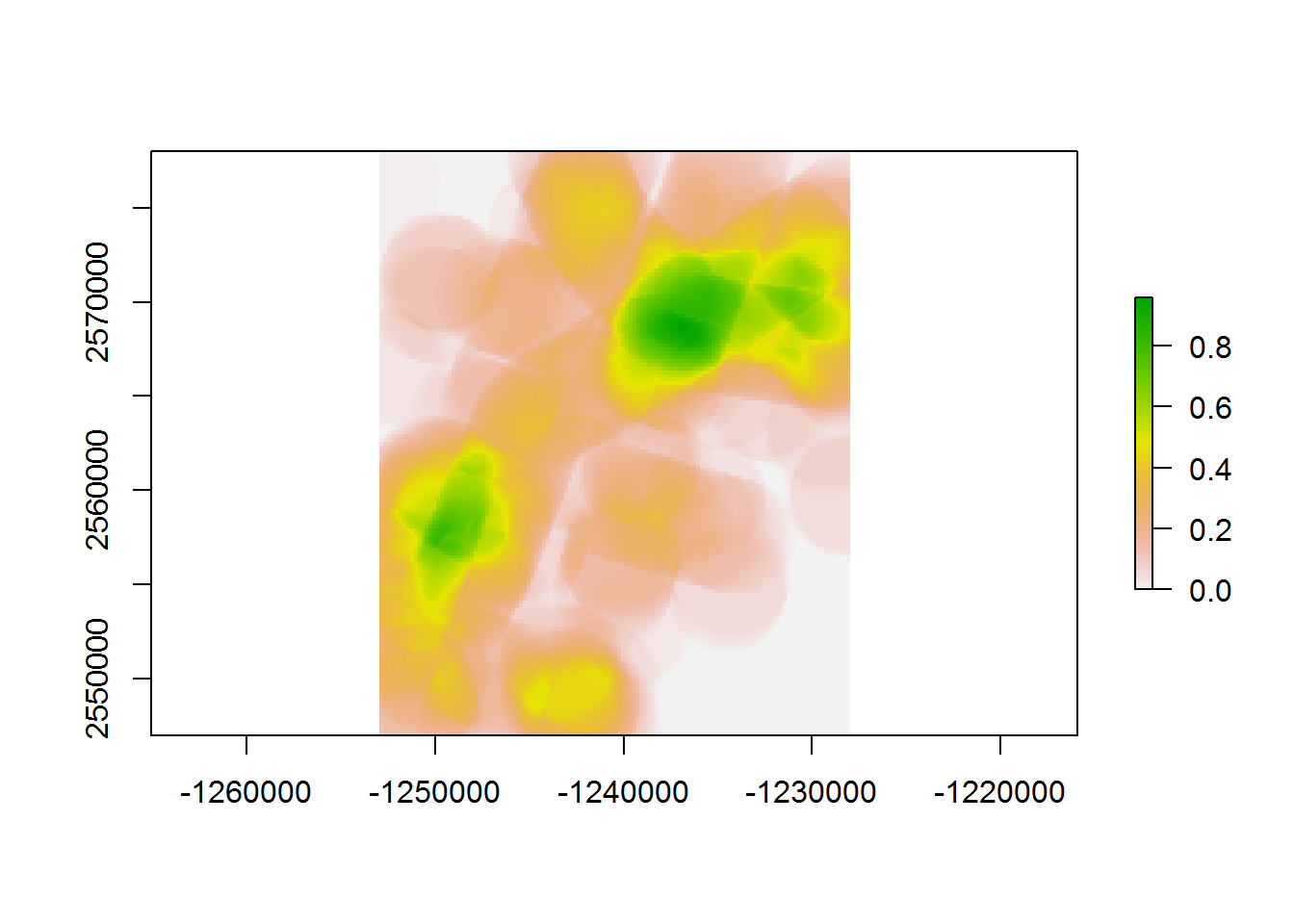
This was slowed considerably by the larger radius, which left few places outside of the analysis.
Let’s run this on the entire dataset at 5km resolution, 10km radius:
system.time(
raster.2km.10km <- makeLineDensityRaster(BEAD.lines, resolution = 2e3, radius = 10e3)
)## user system elapsed
## 38.27 0.14 238.68require(gplots) # for the "rich.colors" palette
plot(raster.2km.10km, col = rich.colors(100))
plot(st_geometry(BEAD.lines), col = "white", add = TRUE)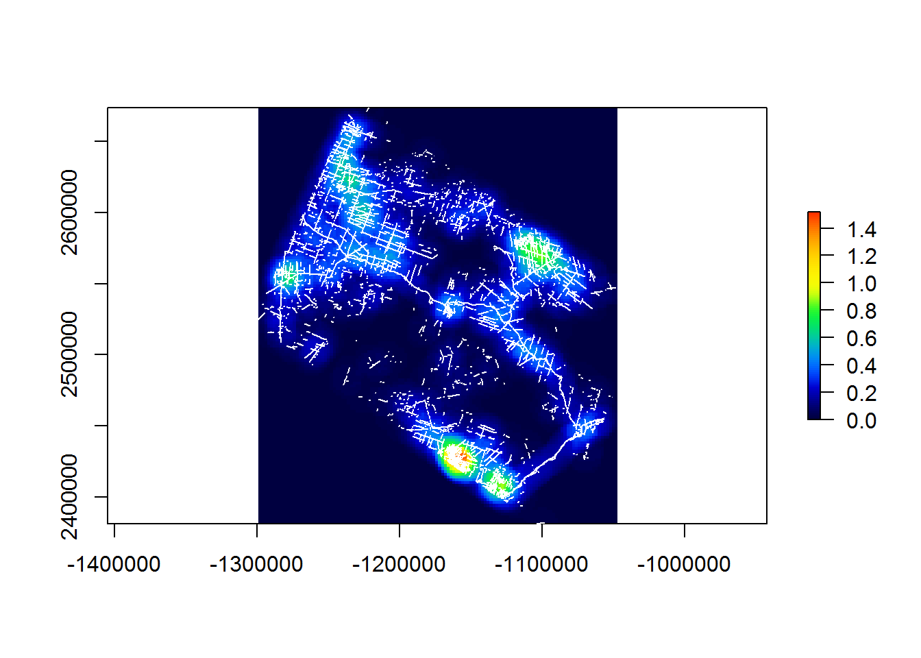
system.time(
raster.2km.5km <- makeLineDensityRaster(BEAD.lines, resolution = 2e3, radius = 5e3)
)## user system elapsed
## 73.03 0.09 268.43require(gplots) # for the "rich.colors" palette
plot(raster.2km.5km, col = rich.colors(100))
plot(st_geometry(BEAD.lines), col = "white", add = TRUE)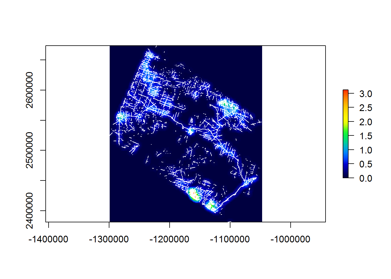
These seem like reasonable times for a landscape-scale computation on a decent laptop with 4 cores. On a more serious machine (e.g, a desktop with 8 or more cores) it is that much faster. It is possible, however, that for the level of resolution that is of actual interest (e.g. < 100m), this is prohibitively slow. One idea - since these are actually very smooth surfaces, is to compute them coarsely and then increase the resolution with a bilinear interpolation via the disaggregate function.
5 Complete code
Click below to show complete code from this document.
knitr::opts_chunk$set(echo = TRUE, cache=TRUE, message = FALSE, warning = FALSE)
par(mar = c(1,1,3,5))
require(sf)
require(raster)
BEAD.lines <- st_read("_data/BEAD/BEADlines2015_NT1_Bistcho_Calendar_MaxH_Yates_HRL_clip.shp")
BEAD.crop <- st_crop(BEAD.lines, extent(-1253e3, -1228e3, 2547e3, 2578e3))
plot(BEAD.crop[,"Class"])
getLineDensity <- function(pt, lines, r, plotme = FALSE){

  pt.circle <- st_buffer(pt, r)
  intersect <- st_intersection(pt.circle, lines)
  length <- sum(st_length(intersect))/1e3 # in km

  density <- (as.numeric(length)/(pi*(r/1e3)^2)) # in km/km^2

  if(plotme){
    plot(st_geometry(lines))
    plot(pt.circle, add = TRUE, border = 2)
    plot(intersect, add = TRUE, col =3)
  }

  return(density)
}
point <- st_point(c(-1240e3, 2560e3), dim = "XY") %>% st_sfc %>% st_sf(crs = st_crs(BEAD.crop))
getLineDensity(point, BEAD.crop, r = 5e3, plotme = TRUE)
getLineDensity(point, BEAD.crop, r = 15e3, plotme = TRUE)
getLineDensity(point, subset(BEAD.crop, Class == "Road"), r = 15e3, plotme = FALSE)
getLineDensity(point, subset(BEAD.crop, Class == "Seismic"), r = 15e3, plotme = FALSE)
density.raster <- raster(extent(BEAD.crop), resolution = 500, crs = st_crs(BEAD.crop))
density.poly <- rasterToPolygons(density.raster)
density.poly.sf <- st_as_sf(density.poly)
st_crs(density.poly.sf) <- st_crs(BEAD.crop)

densities <- rep(NA, nrow(density.poly.sf))
system.time(
  for(i in 1:length(densities))
    densities[i] <- getLineDensity(density.poly.sf[i,], lines = BEAD.crop, r = 1e3, plotme = FALSE)
)
values(density.raster) <- densities
plot(density.raster)
density.poly.list <- split(density.poly.sf, 1:nrow(density.poly.sf))
system.time(
  densities <- sapply(density.poly.list, getLineDensity, lines = BEAD.crop, r = 1e3)
)
values(density.raster) <- densities
plot(density.raster)
r <- 1e3
BEAD.crop.buffered <- st_buffer(BEAD.crop, r) %>% st_union
plot(st_geometry(BEAD.crop.buffered))
which.in.buffer <- st_intersection(st_transform(density.poly.sf, st_crs(BEAD.crop.buffered)), st_geometry(BEAD.crop.buffered)) %>% row.names %>% as.numeric

densities <- rep(0, nrow(density.poly.sf))
density.poly.list <- split(density.poly.sf[which.in.buffer,], 1:length(which.in.buffer))

system.time(
  densities.in.buffer <- sapply(density.poly.list, getLineDensity, lines = BEAD.crop, r = 1e3)
)
values(density.raster)[which.in.buffer] <- densities.in.buffer
plot(density.raster)
## Rprof("_sandbox/Rprofile.out")
## for(i in which.in.buffer)
## densities[i] <- getLineDensity(density.poly.sf[i,], lines = BEAD.crop, r = 1e3)
## Rprof(NULL)
## summaryRprof("_sandbox/Rprofile.out")
require(doParallel)
n <- detectCores()
cl <- makeCluster(n)
clusterEvalQ(cl, library(sf))
clusterExport(cl, "getLineDensity")
system.time(
  densities.in.buffer <- parSapply(cl, density.poly.list, getLineDensity, lines = BEAD.crop, r = 1e3)
  )
values(density.raster)[which.in.buffer] <- densities.in.buffer
plot(density.raster)
stopCluster(cl)
getLineDensity <- function(pt, lines, r, plotme = FALSE){
  pt.circle <- st_buffer(pt, r)
  intersect <- st_intersection(pt.circle, lines)
  length <- sum(st_length(intersect))/1e3
  (as.numeric(length)/(pi*(r/1e3)^2))
}
makeLineDensityRaster <- function(lines, resolution, radius){

  require(raster)
  require(doParallel)
  require(magrittr)
  require(sf)

  # data prep
  density.raster <- raster(extent(lines),
                           resolution = resolution,
                           crs = st_crs(lines))

  density.poly <- rasterToPolygons(density.raster)
  density.poly.sf <- st_as_sf(density.poly)
  st_crs(density.poly.sf) <- st_crs(lines)

  # buffering lines
  lines.buffered <- st_buffer(lines, radius) %>% st_union
  which.in.buffer <- st_intersection(density.poly.sf, lines.buffered) %>%
    row.names %>% as.numeric

  # cluster prep

  density.poly.list <- split(density.poly.sf[which.in.buffer,], 1:length(which.in.buffer))

  cl <- makeCluster(detectCores())
  clusterEvalQ(cl, library(sf))
  clusterExport(cl, "getLineDensity")
  densities.in.buffer <- parSapply(cl, density.poly.list,
                                   getLineDensity, lines = lines, r = radius)
  values(density.raster)[which.in.buffer] <- densities.in.buffer
  density.raster[is.na(density.raster)] <- 0
  stopCluster(cl)
  density.raster
}
system.time(
  raster.200.3km <- makeLineDensityRaster(BEAD.crop, 200, 3e3)
)
plot(raster.200.3km)
system.time(
  raster.2km.10km <- makeLineDensityRaster(BEAD.lines, resolution = 2e3, radius = 10e3)
)
require(gplots) # for the "rich.colors" palette
plot(raster.2km.10km, col = rich.colors(100))
plot(st_geometry(BEAD.lines), col = "white", add = TRUE)
system.time(
  raster.2km.5km <- makeLineDensityRaster(BEAD.lines, resolution = 2e3, radius = 5e3)
)
require(gplots) # for the "rich.colors" palette
plot(raster.2km.5km, col = rich.colors(100))
plot(st_geometry(BEAD.lines), col = "white", add = TRUE)