This is a primer for manipulating a Canada-wide land cover raster of the Northwest Territories. This raster is not as detailed as the EOSD, but it provides an opportuntity to practice manipulating rasters. In particular, we DEFINE and COLLAPSE categorical layers.

1 Load the Land Cover

The land cover raster we are using is from the North American Land Cover Management System (NALCMS), a joint project between Canadian, US, and Mexican organizations. The project is a multi-scale land cover monitoring framework which can be applied across North America. This raster is of a small section of the Northwest Territories, Canada, on the western edge of Great Slave Lake.

Load the raster with the raster command:

require(raster)
landcover <- raster("_data/LandCover/LandCovCanada_c2010_NALCMSlegend_HRL_clip.tif")
landcover

## class      : RasterLayer 
## dimensions : 10290, 10687, 109969230  (nrow, ncol, ncell)
## resolution : 30, 30  (x, y)
## extent     : -1358210, -1037600, 7962570, 8271270  (xmin, xmax, ymin, ymax)
## crs        : +proj=lcc +lat_1=49 +lat_2=77 +lat_0=0 +lon_0=-95 +x_0=0 +y_0=0 +ellps=GRS80 +units=m +no_defs 
## source     : C:/Users/Elie/Box Sync/caribou/NWT/rsf/primers/_data/LandCover/LandCovCanada_c2010_NALCMSlegend_HRL_clip.tif 
## names      : LandCovCanada_c2010_NALCMSlegend_HRL_clip 
## values     : 1, 18  (min, max)
## attributes :
##        ID OBJECTID Value    Count
##  from:  0        1     1 24924814
##   to : 11       12    18  4645750

It plots nicely:

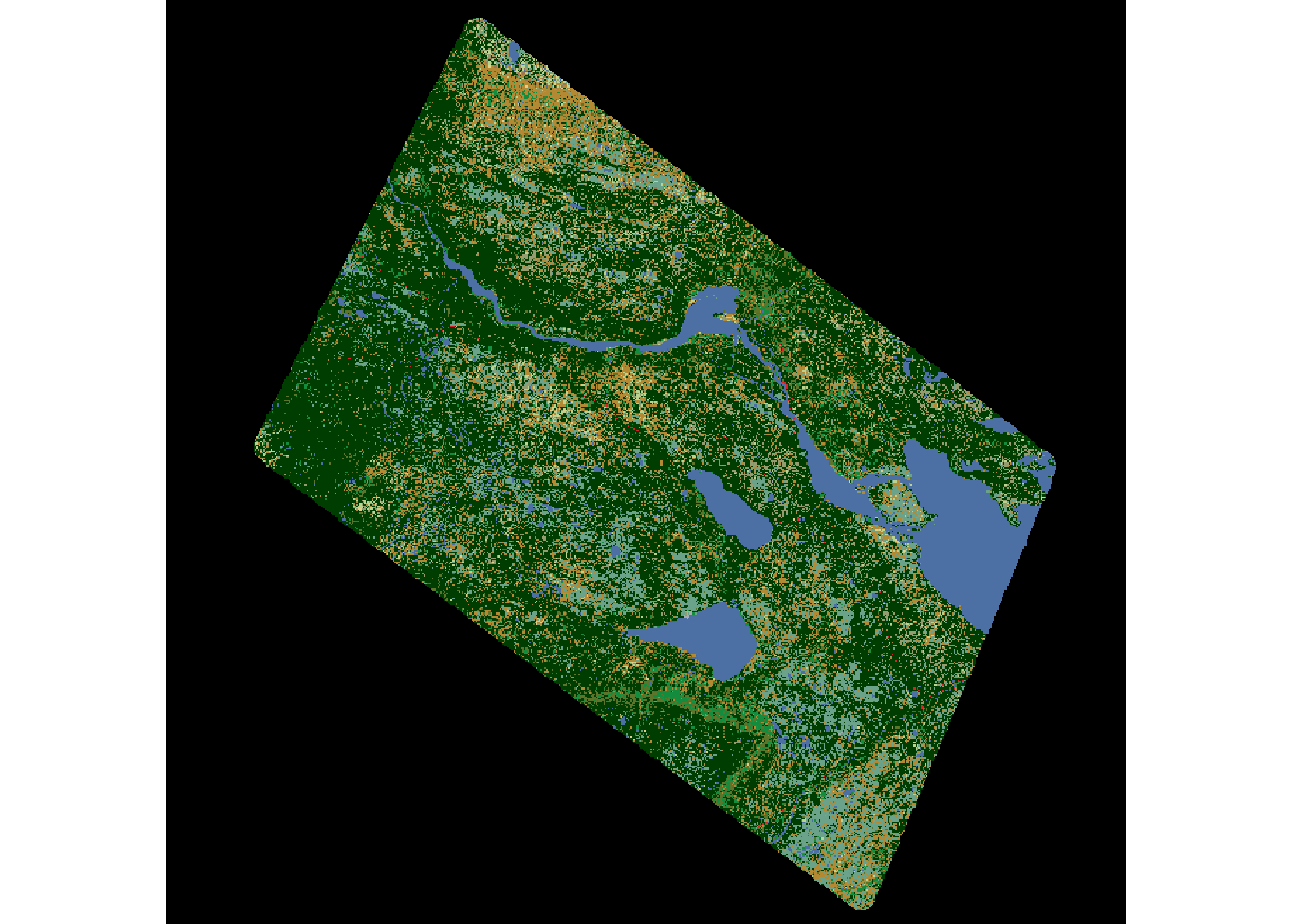
plot(landcover)

But there are no classifications: the raster has an attribute table, but the names of the land cover types are not specified. We need to match up the “Values” to their respective land cover types.

levels(landcover)

## [[1]]
##    ID OBJECTID Value    Count
## 1   0        1     1 24924814
## 2   1        2     2  1973279
## 3   2        3     5  1192339
## 4   3        4     6  2274680
## 5   4        5     8  4593568
## 6   5        6    10    55546
## 7   6        7    11    74603
## 8   7        8    12   692538
## 9   8        9    14  4990755
## 10  9       10    16     7184
## 11 10       11    17    31523
## 12 11       12    18  4645750

These same land cover categories are used throughout the NALCMS dataset, so we can pull the legend from their website: https://landcover.usgs.gov/nalcms.php Unfortunately the legend is in .jpg format, but it’s easy enough to copy into an excel file, which we did manually.

Value	Description	R	G	B
1	Temperate or sub-polar needleleaf forest	0	61	1
2	Sub-polar taiga needleleaf forest	147	156	113
3	Tropical or sub-tropical broadleaf evergreen forest	1	99	0
4	Tropical or sub-tropical broadleaf deciduous forest	29	170	4
5	Temperate or sub-polar broadleaf deciduous forest	19	140	61
6	Mixed Forest	91	117	43
7	Tropical or sub-tropical Shrubland	178	158	43
8	Temperate or sub-polar Shrubland	177	137	50
9	Tropical or sub-tropical Grassland	233	219	94
10	Temperate or sub-polar Grassland	225	206	137
11	Sub-polar or polar shrubland-lichen-moss	156	117	84
12	Sub-polar or polar grassland-lichen-moss	186	211	143
13	Sub-polar or polar barren-lichen-moss	63	137	112
14	Wetland	107	163	136
15	Cropland	230	173	102
16	Barren land	169	170	174
17	Urban	219	33	38
18	Water	76	112	164
19	Snow and Ice	255	248	255

Here is a useful website that can be used to find the specific RGB, HEX or CYMK code of any color in an image. I used it to pull out the RGB code for all the colors in the legend .jpg file: https://www.ginifab.com/feeds/pms/pms_color_in_image.php

2 Add a legend to the Raster:

In order to attach the legend to our raster, we need to merge the levels of the landcover raster with the legend dataframe. Both files have a column named “Value” which we will base the merge on:

levels(landcover)[[1]] <- merge(levels(landcover)[[1]], legend, by = "Value")[,c(2,1,3:5)]

Now we add the colors. The correct colortable is already present in the landcover raster. Here we take the colors in the colortable and add them as a new column in the raster attribute table.(See examples from primer 1)

Note: the raster’s colortable is offset by 1 in relation to our imported legend (the color of the first landcover type is actually the second entry in the list). To keep everything lined up correctly we use Value + 1 instead of just the value.

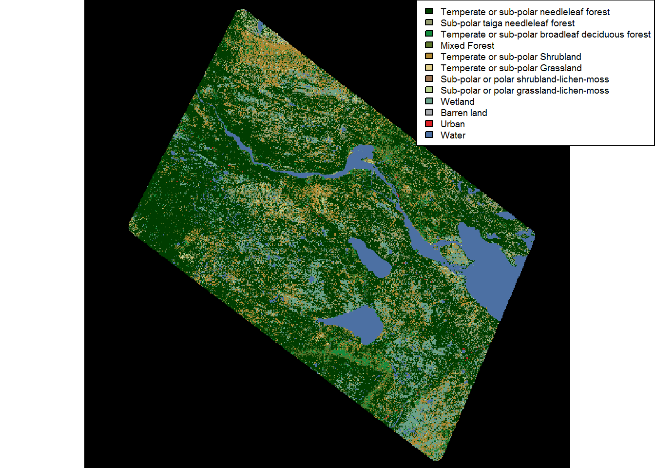
levels(landcover)[[1]]$Colors <- landcover@legend@colortable[levels(landcover)[[1]]$Value + 1]

And there you have it:

plot(landcover)
legend("topright", fill = levels(landcover)[[1]]$Color, legend = levels(landcover)[[1]]$Description, ncol = 1, bg = "white", cex = 0.6)

3 Pool classes together

We have a lot of different land cover types here. To simplify things we can combine similar types into one large land cover category. For example, let’s pool both Temperate or sub-polar needleleaf forest and Sub-polar taiga needleleaf forest (values 17 and 18) into a single class called “1: Needleleaf Forest”.

Steps are simple:

Turn all 2’s into 1’s
Rename 1
Remove row for 2

landcover.pooled <- landcover
values(landcover.pooled)[values(landcover.pooled) == 2] <- 1
mylevels <- levels(landcover.pooled)[[1]]
mylevels$Description <- as.character(mylevels$Description)
mylevels[mylevels$Value == 1,]$Description <- "Needleleaf Forest"
mylevels <- subset(mylevels, Value != 2)
levels(landcover.pooled)[[1]] <- mylevels

To make this more general, e.g. to pool values from a vector sourcevalues to a new value targetvalue and new description newdescription, we write a function:

poolValues <- function(raster, sourcevalues, targetvalue, newdescription){
  raster.pooled <- raster
  values(raster.pooled)[values(raster.pooled) %in% sourcevalues] <- targetvalue
  mylevels <- levels(raster.pooled)[[1]]
  mylevels$Description = as.character(mylevels$Description)
  mylevels[mylevels$Value == targetvalue,]$Description <- newdescription
  mylevels <- subset(mylevels, !(Value %in% sourcevalues) | Value == targetvalue )
  levels(raster.pooled)[[1]] <- suppressWarnings(mylevels)
  return(raster.pooled)
}

Note that this function works on any raster, as long as there is a Description column in the levels.

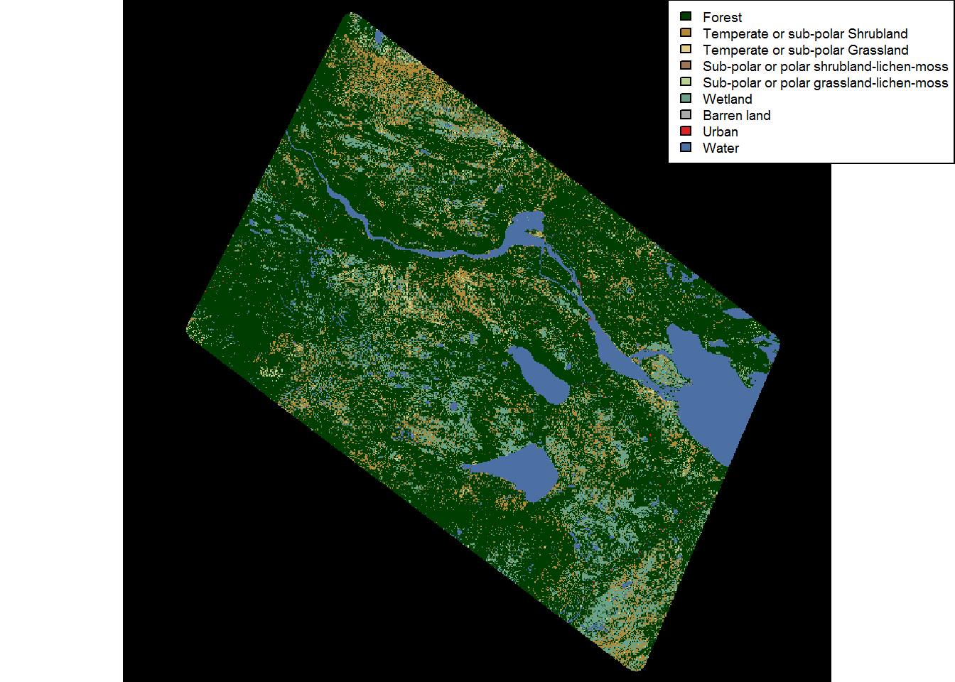
Let’s test this by pooling all of the Forests (classes 1, 2, 5 and 6) into a single monolithic FOREST class:

landcover.forestpooled <- poolValues(landcover, c(1,2,5,6), 1, "Forest")
plot(landcover.forestpooled)
legend("topright", fill = levels(landcover.forestpooled)[[1]]$Color, 
       legend = levels(landcover.forestpooled)[[1]]$Description, 
       ncol = 1, bg = "white", cex = 0.6)

A lot of the forest nuance is now gone! For caribou - probably too much.

	ID	Value	OBJECTID	Count	Description	Colors
1	0	1	1	24924814	Forest	#003D00
5	4	8	5	4593568	Temperate or sub-polar Shrubland	#B38A33
6	5	10	6	55546	Temperate or sub-polar Grassland	#E1CF8A
7	6	11	7	74603	Sub-polar or polar shrubland-lichen-moss	#9C7554
8	7	12	8	692538	Sub-polar or polar grassland-lichen-moss	#BAD48F
9	8	14	9	4990755	Wetland	#6BA38A
10	9	16	10	7184	Barren land	#A8ABAE
11	10	17	11	31523	Urban	#DC2126
12	11	18	12	4645750	Water	#4C70A3

Note: Although there is a column in the dataframe named “Count” this doesn’t actually COUNT anything! Now that multiple rows have been pooled together the count listed in the dataframe isn’t necesarily correct.If you want to know the count (the number of pixels in each land cover category) that would have to be done with the table function (which - for a large raster - can be pretty slow). Below, the count is correct:

levels(landcover.forestpooled)[[1]]$Count <- table(getValues(landcover.forestpooled))

	ID	Value	OBJECTID	Count	Description	Colors
1	0	1	1	30365112	Forest	#003D00
5	4	8	5	4593568	Temperate or sub-polar Shrubland	#B38A33
6	5	10	6	55546	Temperate or sub-polar Grassland	#E1CF8A
7	6	11	7	74603	Sub-polar or polar shrubland-lichen-moss	#9C7554
8	7	12	8	692538	Sub-polar or polar grassland-lichen-moss	#BAD48F
9	8	14	9	4990755	Wetland	#6BA38A
10	9	16	10	7184	Barren land	#A8ABAE
11	10	17	11	31523	Urban	#DC2126
12	11	18	12	4645750	Water	#4C70A3

4 Complete code

Click below to show complete code from this document.

knitr::opts_chunk$set(echo = TRUE, cache=TRUE, message = FALSE, warning = FALSE)
require(raster)
landcover <- raster("_data/LandCover/LandCovCanada_c2010_NALCMSlegend_HRL_clip.tif")
landcover
plot(landcover)
levels(landcover)
require(knitr)
legend <- read.csv("_data/LandCover/NALCMS_Legend.csv")
names(legend)[1] <- "Value"
kable(legend)
levels(landcover)[[1]] <- merge(levels(landcover)[[1]], legend, by = "Value")[,c(2,1,3:5)]
levels(landcover)[[1]]$Colors <- landcover@legend@colortable[levels(landcover)[[1]]$Value + 1]
plot(landcover)
legend("topright", fill = levels(landcover)[[1]]$Color, legend = levels(landcover)[[1]]$Description, ncol = 1, bg = "white", cex = 0.6)
landcover.pooled <- landcover
values(landcover.pooled)[values(landcover.pooled) == 2] <- 1
mylevels <- levels(landcover.pooled)[[1]]
mylevels$Description <- as.character(mylevels$Description)
mylevels[mylevels$Value == 1,]$Description <- "Needleleaf Forest"
mylevels <- subset(mylevels, Value != 2)
levels(landcover.pooled)[[1]] <- mylevels
poolValues <- function(raster, sourcevalues, targetvalue, newdescription){
  raster.pooled <- raster
  values(raster.pooled)[values(raster.pooled) %in% sourcevalues] <- targetvalue
  mylevels <- levels(raster.pooled)[[1]]
  mylevels$Description = as.character(mylevels$Description)
  mylevels[mylevels$Value == targetvalue,]$Description <- newdescription
  mylevels <- subset(mylevels, !(Value %in% sourcevalues) | Value == targetvalue )
  levels(raster.pooled)[[1]] <- suppressWarnings(mylevels)
  return(raster.pooled)
}
landcover.forestpooled <- poolValues(landcover, c(1,2,5,6), 1, "Forest")
plot(landcover.forestpooled)
legend("topright", fill = levels(landcover.forestpooled)[[1]]$Color, 
       legend = levels(landcover.forestpooled)[[1]]$Description, 
       ncol = 1, bg = "white", cex = 0.6)
require(knitr); require(magrittr)
levels(landcover.forestpooled)[[1]] %>% kable
levels(landcover.forestpooled)[[1]]$Count <- table(getValues(landcover.forestpooled))
levels(landcover.forestpooled)[[1]] %>% kable

More Manipulations of Land Cover Raster

Elie and Laura

2019-09-27

1 Load the Land Cover

2 Add a legend to the Raster:

3 Pool classes together

4 Complete code