Movement and Rasters
Elie Gurarie and Laura Berman
UPDATED: 2019-04-16
Goals:
Calculate proportion of each land cover class within a 1 km buffer around each collar location; or calculate dominant land cover type within that buffer; or diversity of land cover types within that buffer.
List of required packages for these tasks (the code below will load all of them):
pcks <- c("move", "raster", "sf", "ggplot2", "plyr", "scales", "lubridate")
a <- sapply(pcks, require, character = TRUE)
1 Load and process South Slave movement data
Loading the South Slave Boreal Woodland Caribou data set.
southies <- getMovebankData("ABoVE: NWT South Slave Boreal Woodland Caribou", login = mylogin)There are:
nrow(southies@idData)## [1] 201individuals in this data set.
I’ll convert this to a data frame, which is (for many things) easier to work with:
southies.df <- as.data.frame(southies)This is a data frame like object, which is very convenient for manipulation. In this primer, I will also use the magrittr pipe (%>%) syntax, which is a way of coding that allows for a more “natural” syntax, instead of stacking functions outwards: dof4(dof3(dof2(dof1(data)))), it allows you to write the same thing in a more logical string: data %>% dof1 %>% dof2 %>% dof3 %>% dof4. THe convenience of this - in particular for data frames - should be evident by example.
Here is a plot of the duration of the data by time (a useful visualization):
require(magrittr) # for piping
require(plyr) # for data frame manipulation
southies.timerange <- southies.df %>% ddply(c("nick_name","habitat"), summarize,                                                                                     start = min(timestamp), end = max(timestamp)) %>%
    plyr::arrange(habitat,start) %>%
    mutate(nick_name = as.factor(1:length(unique(nick_name))))

# this last line of code is just to make the ordering work right in the figure below

require(ggplot2)
ggplot(southies.timerange, aes(x = start, y = nick_name, col = habitat)) +
    geom_segment(aes(x = start, xend = end, yend = nick_name)) + theme_bw()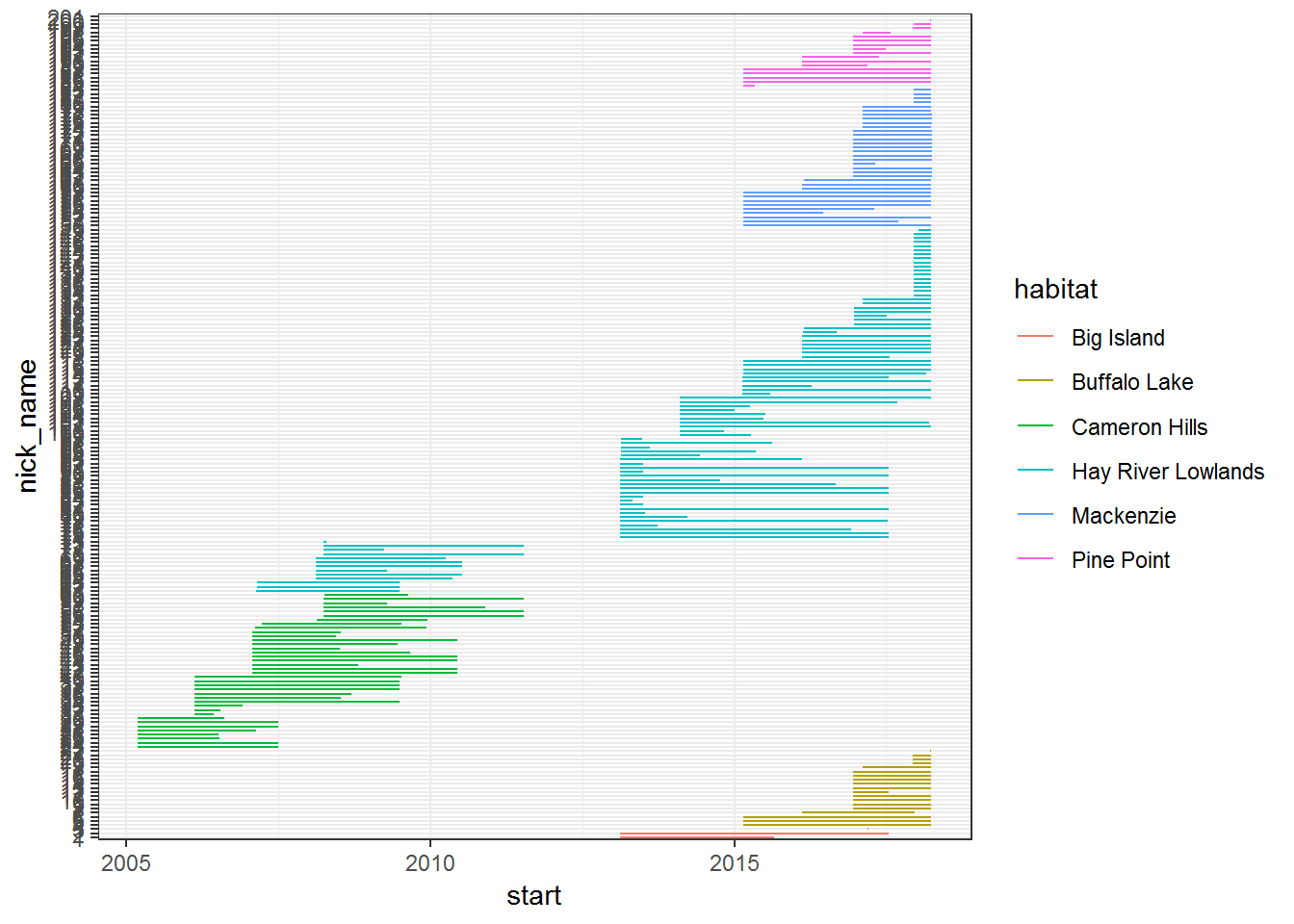
We can see (for example) that there was a gap in the coverage somewhere between 2012 and 2014, and that Cameron Hills is entirely on the earlier end of the gap. Also, it can be interesting (for other, mortality related reasons) to look at the duration of the collars transmitting pre-drop-off.
Plotting all location data:
ggplot(southies.df, aes(location_long, location_lat, col = habitat)) + geom_path() + theme_bw()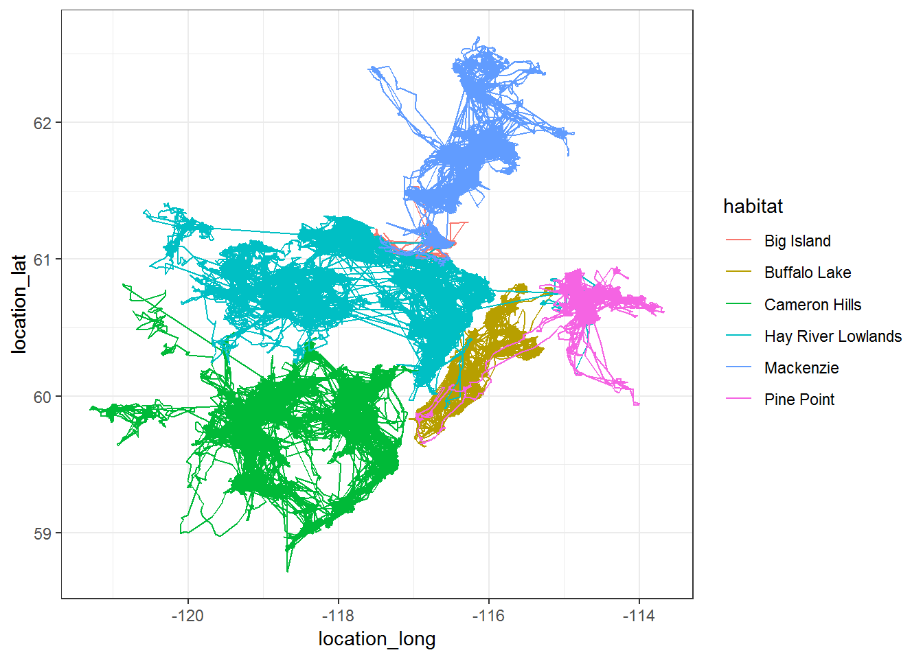
Note the projection of these data is latlong WGS84:
southies@proj4string## CRS arguments:
## +proj=longlat +ellps=WGS84 +datum=WGS84 +towgs84=0,0,02 Linking movement and Land cover raster
2.1 Loading the raster
Load the raster from previous exercise:
eosd <- raster("./_data/rasters/EOSD_withfire")plot(eosd)
legend("topright", fill = levels(eosd)[[1]]$Color,
legend = levels(eosd)[[1]]$Description, ncol = 2, cex = 0.55)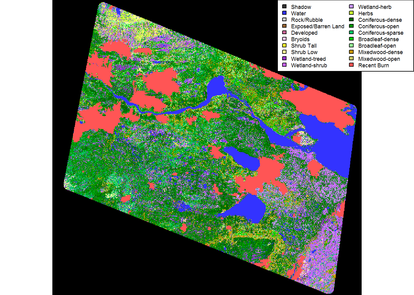
2.2 Plot movement on raster
Now we plot one on top the other, to be sure that they are correctly projected. We’ll focus on the Hay River Lowlands group (and - just to make things simpler - only on those tagged BEFORE 2012), but we need to (a) reproject to the raster and (b) subset those from the original movement data. Some of these things are easier to do with simple feature objects. Note the piping in the (single) command below:
require(lubridate) # for the ymd function below
hayriver.sf <- southies.df %>% subset(habitat == "Hay River Lowlands" & timestamp < ymd("2012-01-01")) %>%
st_as_sf(coords = c("location_long", "location_lat"), crs = projection(southies)) %>% st_transform(projection(eosd)) There are a few functions in that (single) line of code that are specific to “simple features”. These functions all start with st_, most important: st_transform which quickly transforms the data to the projection of the raster.
plot(eosd)
nick_names <- unique(hayriver.sf$nick_name)
greys <- grey(seq(.5,1,length = length(nick_names)))
for(i in 1:length(nick_names)){
xy <- st_coordinates(subset(hayriver.sf, nick_name == nick_names[i]))
lines(xy, col = greys[i])
}
3 Extracting variables
To find out what landscape type each individual location is ON is extremely easy (in contrast to what follows) and surprisingly fast. All you need is the “extract” command. First make sure the projections match:
crs(hayriver.sf)## [1] "+proj=aea +lat_1=50 +lat_2=70 +lat_0=40 +lon_0=-112 +x_0=0 +y_0=0 +ellps=GRS80 +towgs84=0,0,0,0,0,0,0 +units=m +no_defs"crs(eosd) ## CRS arguments:
## +proj=aea +lat_1=50 +lat_2=70 +lat_0=40 +lon_0=-112 +x_0=0 +y_0=0
## +datum=NAD83 +units=m +no_defs +ellps=GRS80 +towgs84=0,0,0Now, extract:
hayriver.landcover <- raster::extract(eosd, st_coordinates(hayriver.sf))table(hayriver.landcover)## hayriver.landcover
## 0 20 40 52 81 82 83 211 212 213 221 222 231 232 250
## 81 91 3 32 724 1404 682 1373 3174 460 3 6 164 72 650The only nuance here is that raster doesn’t work well (yet) with simple features, so we had to extract the coordiantes of from the hayriver.sf object using the st_coordinates function.
The result IS the landclass for each location, BUT it is coded as numeric and corresponds to the vector of landclass colors summarized in the “Value” column of the attributes table:
levels(eosd)## [[1]]
## ID OBJECTID Value Description Color Count
## 1 0 1 12 Shadow #333333 365
## 2 1 2 20 Water #3333FF 5559064
## 3 2 3 32 Rock/Rubble #CCCCCC 67
## 4 3 4 33 Exposed/Barren Land #996633 13635
## 5 4 5 34 Developed #CC6699 64239
## 6 5 6 40 Bryoids #FFCCFF 96789
## 7 6 7 51 Shrub Tall #FFFF33 72952
## 8 7 8 52 Shrub Low #FFFF99 668629
## 9 8 9 81 Wetland-treed #9933CC 2358766
## 10 9 10 82 Wetland-shrub #CC66FF 4242600
## 11 10 11 83 Wetland-herb #CC99FF 1160373
## 12 11 12 100 Herbs #CCFF33 514846
## 13 12 13 211 Coniferous-dense #006600 6715586
## 14 13 14 212 Coniferous-open #009900 11162064
## 15 14 15 213 Coniferous-sparse #00CC66 3236051
## 16 15 16 221 Broadleaf-dense #00CC00 917321
## 17 16 17 222 Broadleaf-open #99FF99 985631
## 18 17 18 231 Mixedwood-dense #CC9900 3088338
## 19 18 19 232 Mixedwood-open #CCCC66 600763
## 20 19 20 250 Recent Burn #FF5555 67316953.1 Three barplots
Here are some barplots:
hayriver.landclass <- with(levels(eosd)[[1]], Description[match(hayriver.landcover, Value)])
par(mar = c(3,10,2,2))
barplot(table(hayriver.landclass), horiz = TRUE, las = 1)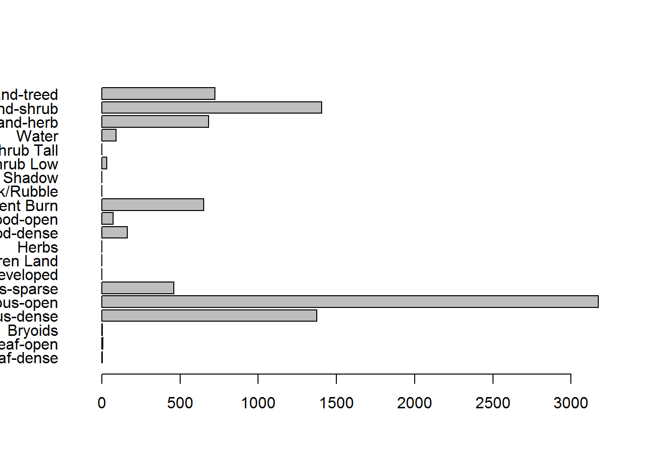
count.df <- data.frame(Description = names(table(hayriver.landclass)),
CaribouCount = table(hayriver.landclass) %>% as.numeric) %>% merge(
levels(eosd)[[1]][,c("Description","Color","Count")])
par(mar = c(3,10,2,2))
with(arrange(count.df, CaribouCount),
barplot(CaribouCount, horiz = TRUE, las = 1, col = Color, names.arg = Description))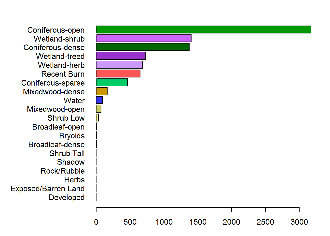
Comparing “used” and “available”
count.df$p.Used <- prop.table(count.df$CaribouCount)
count.df$p.Available <- prop.table(count.df$Count)
par(mar = c(3,10,2,2))
with(arrange(count.df, CaribouCount),
barplot(rbind(p.Used, p.Available), horiz = TRUE, las = 1, beside = TRUE, bor = NA,
col = rbind(alpha(Color, 0.5), Color),
axes = FALSE))
mtext(side = 2, at = seq(3,60,3) - .5,
text = arrange(count.df, CaribouCount)$Description, las = 1, cex = 0.7)
legend("bottomright", fill = c("black","grey"), legend = c("available", "used"), bty = "n")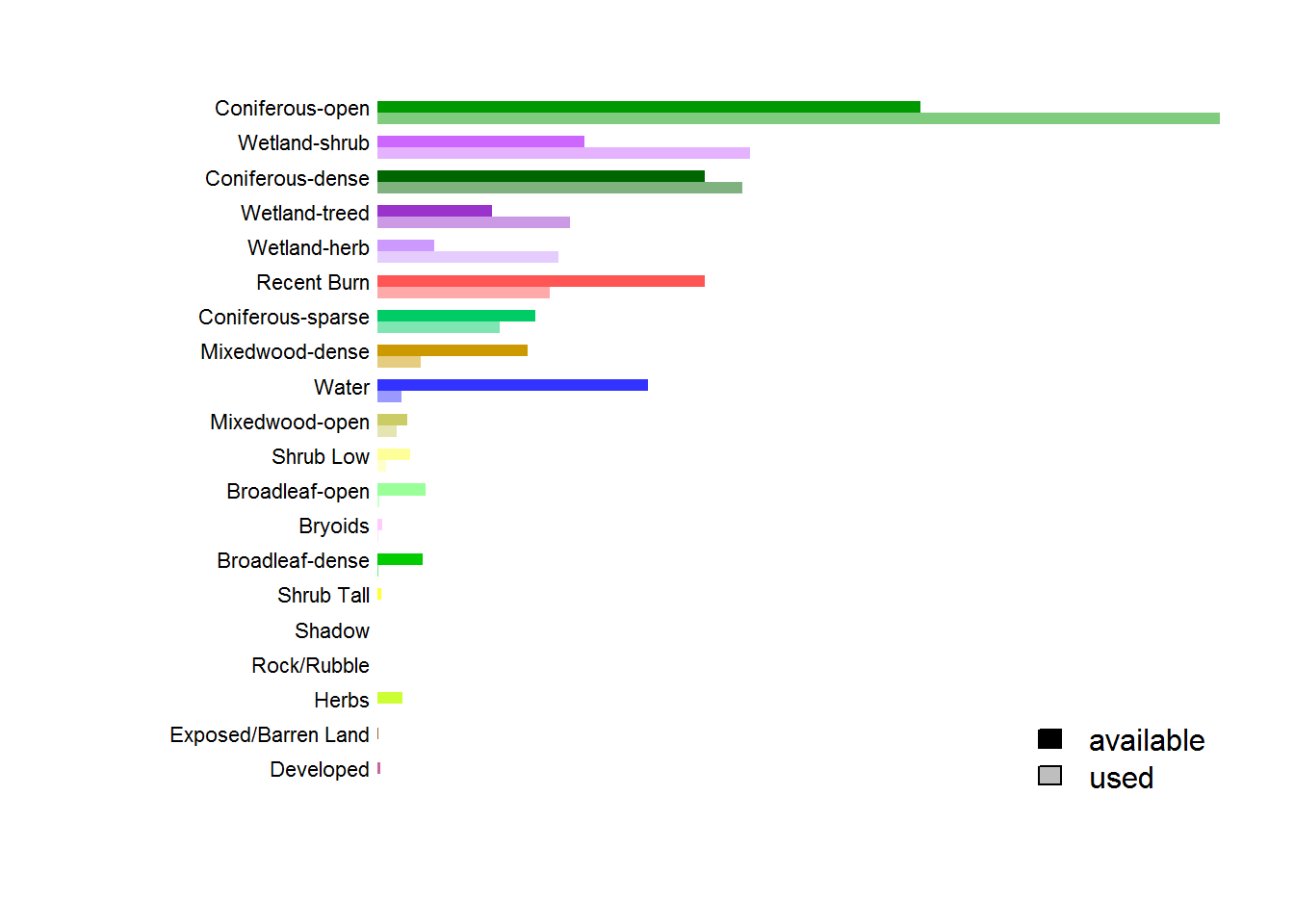
Just from this plot, there is a clear preference for coniferous-open and wetland shrub habitats, and an avoidance of (obviously) water, but (more relevantly) recent burns, and broadleaf habitats.
4 Extracting from a buffer
The task of computing the land classes within a radius of a given location is best considered by zooming way down to a single location. Let’s draw the EOSD in a 1 km buffer around the first location:
extent(hayriver.sf[1,])## class : Extent
## xmin : -258895.2
## xmax : -258895.2
## ymin : 2255298
## ymax : 2255298(crop.extent <- extent(hayriver.sf[1,]) + 2e3 * c(-1,1,-1,1))## class : Extent
## xmin : -260895.2
## xmax : -256895.2
## ymin : 2253298
## ymax : 2257298eosd.cropped <- crop(eosd, crop.extent)
plot(eosd.cropped)
plot(st_geometry(hayriver.sf[1,]), col = "black", lwd = 2, cex = 3, pch = 21, bg = "white", add = TRUE)
xy <- st_coordinates(hayriver.sf[1,])[1,]
radius <- 1e3
z.circle <- (xy[1] + 1i*xy[2]) + complex(mod = radius, arg = seq(0, 2*pi, length = 1000))
circle.sf <- st_polygon(x = list(cbind(X = Re(z.circle), Y = Im(z.circle))))
plot(st_geometry(circle.sf), add = TRUE, col = rgb(1,1,1,.3))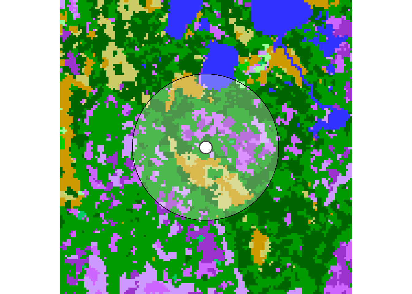
Note, the way I drew the circle (with the possibly odd-looking (xy[1] + 1i*xy[2]) + complex(...)) was to use so called “complex numbers”, which make dealing with 2d vectors very easy once you get used to them. Here is a link to a lecture on using complex numbers in the more specific context of animal movement data.
We’re going to consider 2 different summaries: (1) The most common lancover type, (2) the complete “community”.
4.1 Most common type in a buffer
This is the most straightforward, since the extract function can extract from a buffer:
raster::extract(eosd, hayriver.sf[1,], buffer = 1000, fun = function(x) which.max(tabulate(x)))## [1] 212The top value within 1k buffer is 212, which (cross-checking with the attributes table):
levels(eosd)## [[1]]
## ID OBJECTID Value Description Color Count
## 1 0 1 12 Shadow #333333 365
## 2 1 2 20 Water #3333FF 5559064
## 3 2 3 32 Rock/Rubble #CCCCCC 67
## 4 3 4 33 Exposed/Barren Land #996633 13635
## 5 4 5 34 Developed #CC6699 64239
## 6 5 6 40 Bryoids #FFCCFF 96789
## 7 6 7 51 Shrub Tall #FFFF33 72952
## 8 7 8 52 Shrub Low #FFFF99 668629
## 9 8 9 81 Wetland-treed #9933CC 2358766
## 10 9 10 82 Wetland-shrub #CC66FF 4242600
## 11 10 11 83 Wetland-herb #CC99FF 1160373
## 12 11 12 100 Herbs #CCFF33 514846
## 13 12 13 211 Coniferous-dense #006600 6715586
## 14 13 14 212 Coniferous-open #009900 11162064
## 15 14 15 213 Coniferous-sparse #00CC66 3236051
## 16 15 16 221 Broadleaf-dense #00CC00 917321
## 17 16 17 222 Broadleaf-open #99FF99 985631
## 18 17 18 231 Mixedwood-dense #CC9900 3088338
## 19 18 19 232 Mixedwood-open #CCCC66 600763
## 20 19 20 250 Recent Burn #FF5555 6731695is “Coniferous Open”.
Here’s the most common habitat type for the complete data set. To save time, I only do the first individual (hr108):
hr108 <- subset(hayriver.sf, nick_name == "HR108")
system.time(
landcover.mode <- raster::extract(eosd, hr108, buffer = 1000, fun = function(x) which.max(tabulate(x)))
)## user system elapsed
## 2.56 0.11 2.67That’s quite quick! Here’s the table:
table(landcover.mode)## landcover.mode
## 20 81 82 83 211 212 231 250
## 9 5 18 3 30 337 9 44And a color coded barplot referring to the EOSD attributes):
levels <- levels(eosd)[[1]]
hr108.levels <- levels[match(names(table(landcover.mode)), levels$Value),]
hr108.levels## ID OBJECTID Value Description Color Count
## 2 1 2 20 Water #3333FF 5559064
## 9 8 9 81 Wetland-treed #9933CC 2358766
## 10 9 10 82 Wetland-shrub #CC66FF 4242600
## 11 10 11 83 Wetland-herb #CC99FF 1160373
## 13 12 13 211 Coniferous-dense #006600 6715586
## 14 13 14 212 Coniferous-open #009900 11162064
## 18 17 18 231 Mixedwood-dense #CC9900 3088338
## 20 19 20 250 Recent Burn #FF5555 6731695barplot(table(landcover.mode), col = hr108.levels$Color,
legend.text = hr108.levels$Description, args.legend=list(x = "topleft"))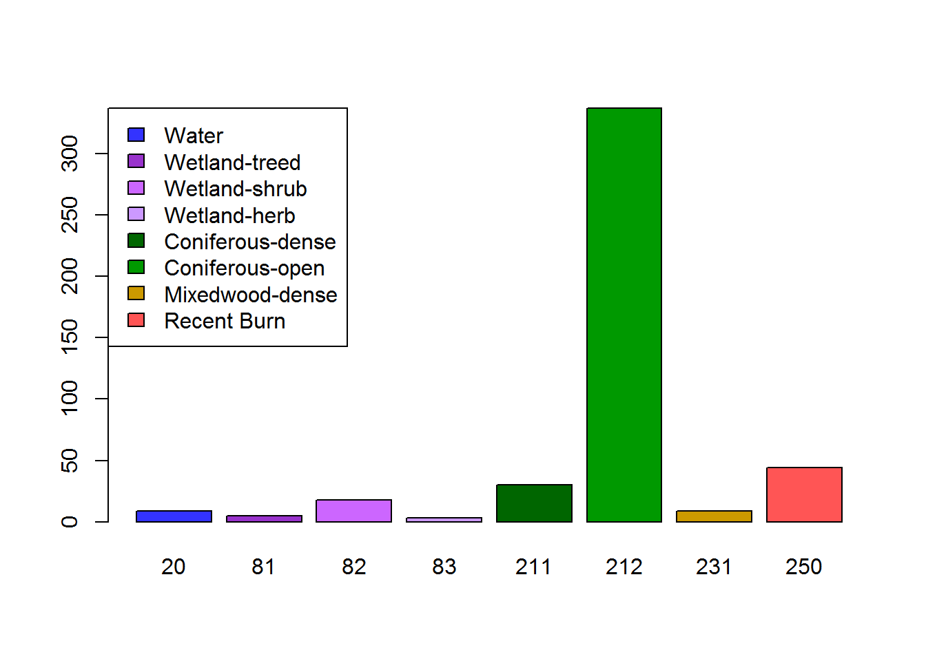
4.2 Complete community in a buffer
4.2.1 Buffering with raster::mask (inefficient but instructive)
(Really you should skip to the next section, which is much, much faster)
To characterize the complete habitat data around this point, we need to:
- draw a circle
- turn it in to a polygon
- “mask” the raster with the circle
- count the remaining points
The key function is mask:
eosd.masked <- mask(eosd.cropped, as(circle.sf, "Spatial"))
plot(eosd.masked)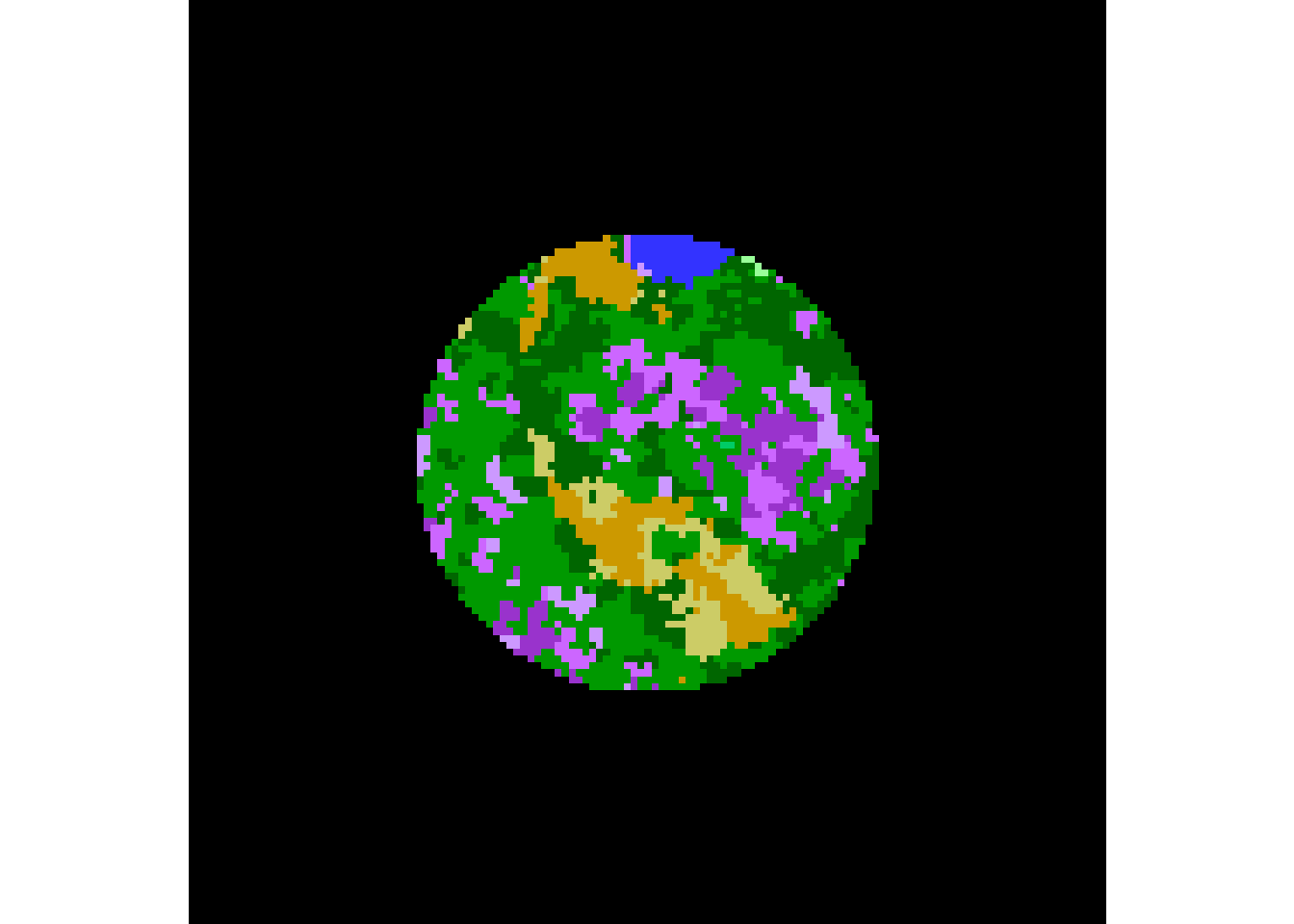
table(getValues(eosd.masked))##
## 20 81 82 83 211 212 213 222 231 232
## 78 247 321 119 834 1347 2 5 325 212This process (the circle from above and the masking) needs to be replicated for every point. Most efficiently, we write a little function that returns just this table for any given (simple feature) point, e.g.:
getLandcoverInBuffer <- function(xy, radius){
xy <- st_coordinates(xy)[1,]
crop.extent <- xy + radius * c(-1,1,-1,1)
eosd.cropped <- crop(eosd, crop.extent)
z.circle <- (xy[1] + 1i*xy[2]) + complex(mod = radius, arg = seq(0, 2*pi, length = 1000))
circle.sf <- st_polygon(x = list(cbind(X = Re(z.circle), Y = Im(z.circle))))
eosd.masked <- mask(eosd.cropped, as(circle.sf, "Spatial"))
table(getValues(eosd.masked))
}
getLandcoverInBuffer(hayriver.sf[1,], 1e3)##
## 20 81 82 83 211 212 213 222 231 232
## 78 247 321 119 834 1347 2 5 325 212getLandcoverInBuffer(hayriver.sf[5,], 1e3)##
## 20 81 82 83 211 212 213 231 232
## 530 224 211 130 606 1436 101 223 32This is unappealingly slow, even for a single point (on my decent laptop):
system.time(getLandcoverInBuffer(hayriver.sf[1,], 1e3))## user system elapsed
## 1.50 0.10 1.61It takes 1.7 seconds per point. We have 9000 thousand points just in Hay River, so the complete process would take over 4 hours just for that one data subset, so not very practical. Still, to illustrate how to scale up, here’s a loop applied to just the first 30 locations from animal hr108):
hr108 <- subset(hayriver.sf, nick_name == "HR108")[1:30,]The loop
# initialize matrix with 250(!) columns for each possible value to populate with results of the table count
landcover.matrix <- matrix(NA, nrow = nrow(hr108), ncol = 250)
system.time(
for(i in 1:nrow(hr108)){
my.lcs <- getLandcoverInBuffer(hayriver.sf[i,], 1e3)
which <- as.numeric(names(my.lcs))
landcover.matrix[i,which] <- as.numeric(my.lcs)
})The loop generated a matrix of counts. Let’s (a) compute the proportions, (b) make it a data frame, (c) remove all the empty columns:
# apply runs a function across dimensions (in this case 1 = rows) of a matrix ... unfortunately it also turns it sideways (in this case), hence the `t` at the end
p.landcover.matrix <- apply(landcover.matrix, 1, function(x) x/(sum(x, na.rm = TRUE))) %>% t
# change the NA's to 0's
p.landcover.matrix[is.na(p.landcover.matrix)] <- 0
data_columns <- colSums(p.landcover.matrix) > 0
p.landcover.df <- data.frame(p.landcover.matrix[,data_columns])
names(p.landcover.df) <- which(data_columns)
head(p.landcover.df)## 20 52 81 82 83 211 212
## 1 0.02234957 0 0.07077364 0.09197708 0.03409742 0.23896848 0.3859599
## 2 0.03697334 0 0.21553454 0.20865578 0.02579536 0.13814847 0.3419318
## 3 0.00000000 0 0.02004008 0.06097910 0.08559977 0.20269110 0.4660750
## 4 0.11712486 0 0.25429553 0.11683849 0.08963345 0.07187858 0.3399198
## 5 0.15173204 0 0.06412826 0.06040653 0.03721729 0.17348984 0.4111079
## 6 0.13925501 0 0.17220630 0.04183381 0.05243553 0.09828080 0.4103152
## 213 221 222 231 232
## 1 0.0005730659 0.0000000000 0.001432665 0.093123209 0.0607449857
## 2 0.0266552021 0.0000000000 0.000000000 0.004872456 0.0014330754
## 3 0.0134554824 0.0002862869 0.002004008 0.121099342 0.0277698254
## 4 0.0088774341 0.0000000000 0.000000000 0.000000000 0.0005727377
## 5 0.0289149728 0.0000000000 0.000000000 0.063841970 0.0091611795
## 6 0.0340974212 0.0000000000 0.000000000 0.048137536 0.0034383954
## 250
## 1 0.0000000000
## 2 0.0000000000
## 3 0.0000000000
## 4 0.0008591065
## 5 0.0000000000
## 6 0.0000000000Here’s an illustration of what the caribou experienced in time. We have to fuss around a bit with the attributes column to match the colors to the right classes:
levels <- levels(eosd)[[1]]
legend.table <- levels[match(names(p.landcover.df), levels$Value), ]
matplot(hr108$timestamp, p.landcover.df, type="o", pch = 19, lty = 1,
col = legend.table$Color, lwd = 1, xlab = "time", xaxt="n", ylim = c(0,1))
# some non-intuitive code to make the x-axis show times correctly
axis(1, at = pretty(hr108$timestamp), labels = as.character(pretty(hr108$timestamp)))
legend("top", col = legend.table$Color, pch = 19, lty = 1, legend = legend.table$Description, ncol = 3, cex = 0.8, bty = "n")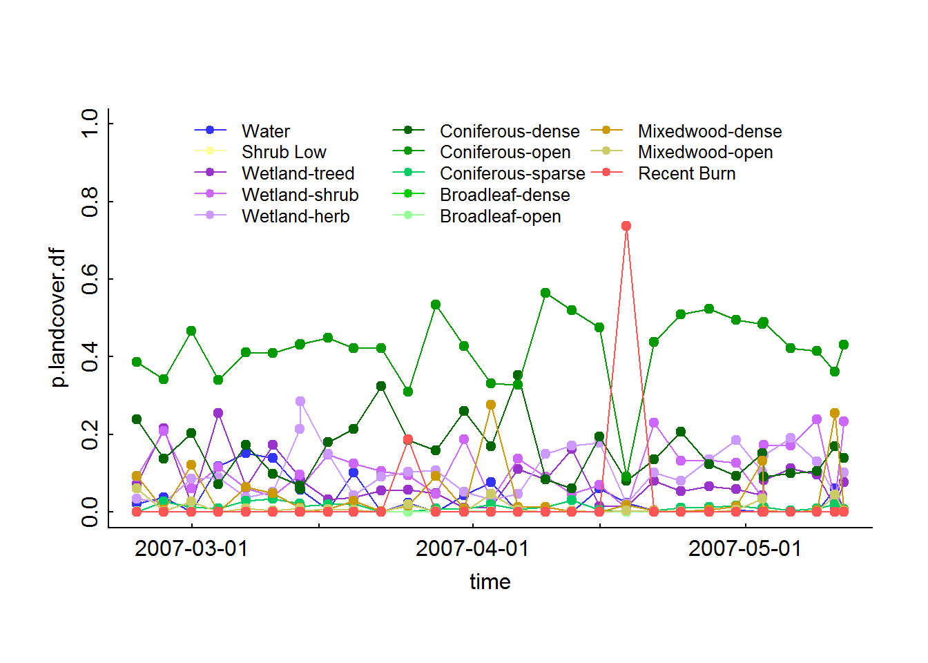
This animal hangs out around a lot of confirous open habitat, with one brief foray into a recent fire (though - it’s not entirely clear that that fire was ACTUALLY more recent than when the caribou was in there).
Here’s another (better?) visualization:
time <- hr108$timestamp
ddays <- difftime(time[-1], time[-nrow(hr108)], units = "days") %>% as.numeric
barplot(p.landcover.df %>% t %>% as.matrix, space = 0,
width = c(0,ddays),
col = legend.table$Color, bor = NA, sep = 0)
totaltime <- difftime(max(time), min(time), units= "days")
axis(1, at = difftime(pretty(time, n = 10), min(time), units = "days"),
labels = as.character(pretty(time, n = 10)))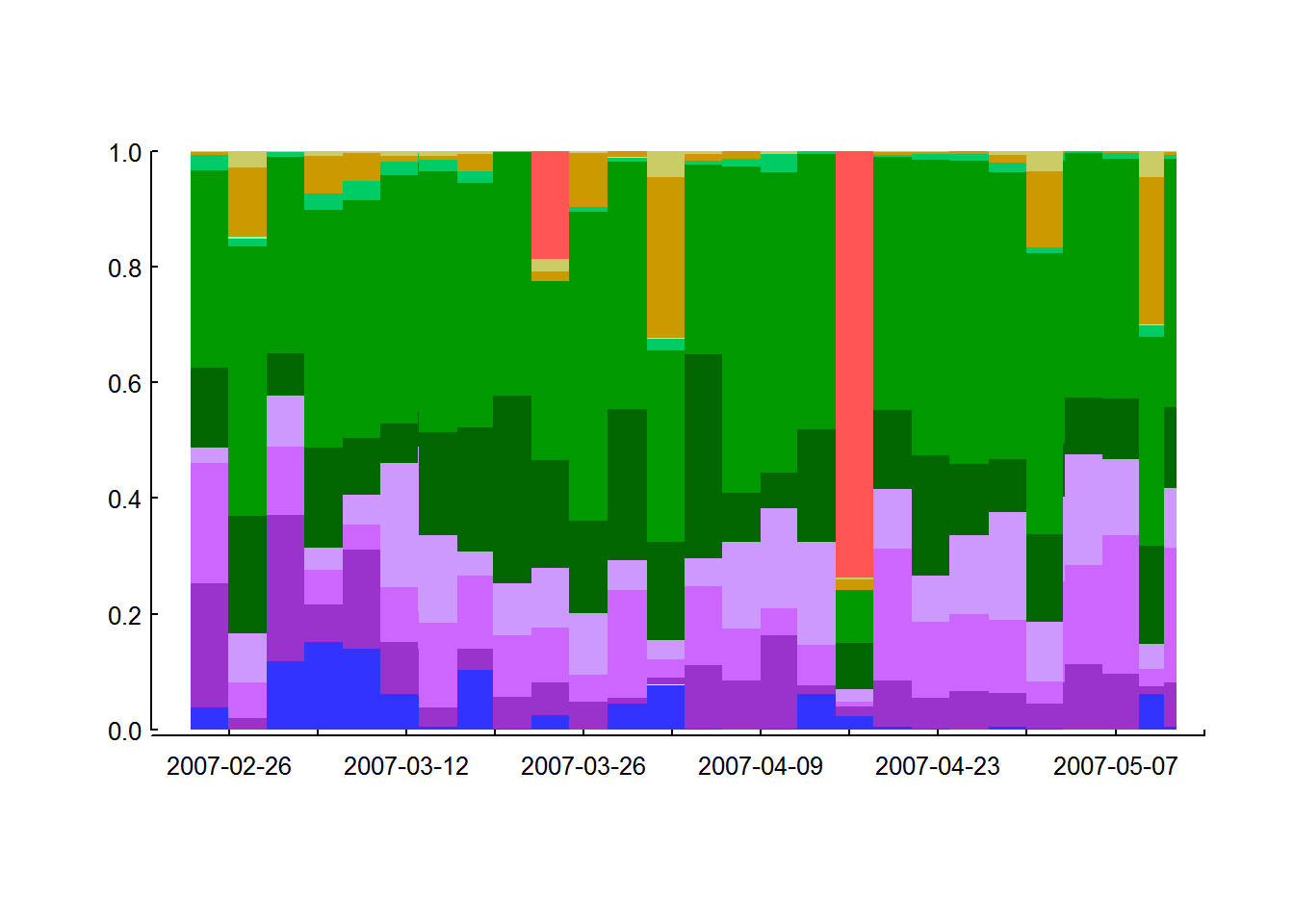
Anyways - this method is too slow. But the visualizations may prove useful later.
4.2.2 Buffering with raster::extract (much faster)
We can use the buffered extract function (see preceding subsection) to count each of the possible values, and stack those into a matrix. I do the stacking with sapply() - a powerful base function to do loops without writing loops - applying across the possible vlaues of eosd. I do this below for the complete hr108 data set, and time it:
hr108 <- subset(hayriver.sf, nick_name == nick_name[1])
eosd.values <- levels(eosd)[[1]]$Value
system.time(
landcover2.matrix <- sapply(eosd.values,
function(v) raster::extract(eosd, hr108, buffer = 1e3, fun = function(x) sum(x == v)))
)## user system elapsed
## 62.60 3.40 68.09This only took 1 minute! Compare to the 12 minutes it would have taken using the method above.
Now that these are computed, we (a) name the columns to be the names of the data levels, and (b) compute the proportion use against time:
colnames(landcover2.matrix) <- eosd.values
p.landcover2.df <- apply(landcover2.matrix, 1, function(x) x/(sum(x, na.rm = TRUE))) %>% t %>% as.data.frameHere is the complete 1km landcover buffered community for this individual by time:
Collecting useful bits:
time <- hr108$timestamp
ddays <- difftime(time[-1], time[-nrow(hr108)], units = "days") %>% as.numeric
eosd.levels <- levels(eosd)[[1]]
hr108.levels <- eosd.levels[match(names(p.landcover2.df), eosd.levels$Value),]Barplot:
barplot(p.landcover2.df %>% t %>% as.matrix, space = 0,
width = c(0,ddays), legend.text = hr108.levels$Description, args.legend=list(cex = 0.7, bty = "n"),
col = hr108.levels$Color, bor = NA, sep = 0,
xlim = c(0,sum(ddays)*1.3))
totaltime <- difftime(max(time), min(time), units= "days")
axis(1, at = difftime(pretty(time, n = 10), min(time), units = "days"),
labels = as.character(pretty(time, n = 10)))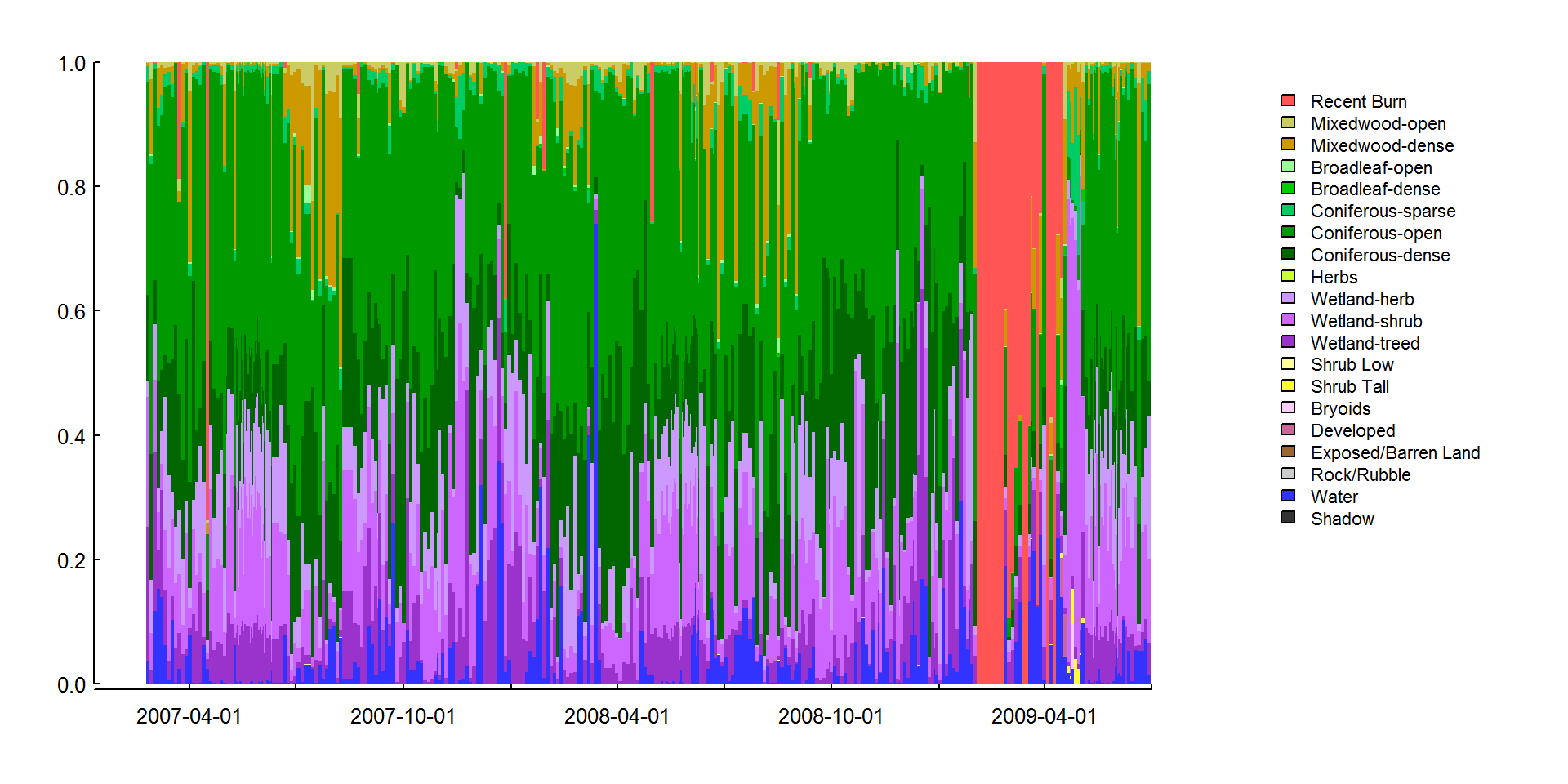
Here it’s worth noting that with the apply functions, there are opportunities to parallelize the code, i.e. use multiple cores on your computer. Here’s an example repeating the above operation:
# key package (though there are others)
library(parallel)
# generate the cluster. THe 4 is the number of cores on my laptop, but I have, e.g., 8 on my desktop, for example.
cl = makeCluster(4)
# important for all the cores to have access to the raster, the movement data, and the raster package:
clusterExport(cl, list('eosd','hr108'))
clusterEvalQ(cl, library(raster))## [[1]]
## [1] "raster" "sp" "stats" "graphics" "grDevices" "utils"
## [7] "datasets" "methods" "base"
##
## [[2]]
## [1] "raster" "sp" "stats" "graphics" "grDevices" "utils"
## [7] "datasets" "methods" "base"
##
## [[3]]
## [1] "raster" "sp" "stats" "graphics" "grDevices" "utils"
## [7] "datasets" "methods" "base"
##
## [[4]]
## [1] "raster" "sp" "stats" "graphics" "grDevices" "utils"
## [7] "datasets" "methods" "base"# do a parallel sapply:
system.time(
hr2 <- parSapply(cl, eosd.values,
function(v) raster::extract(eosd, hr108, buffer = 1e3,
fun = function(x) sum(x == v)))
)## user system elapsed
## 0.00 0.00 27.46This speeded up the process by a factor (nearly) of 4, as expected, since that’s the number of cores I put to work.
4.3 Buffering the spatial line
A third option is to buffer the movement track itself, and mask that from the raster. This is the fastest option, but only useful if you don’t care at all about the temporal structure, i.e. you’ll get a single spatial count of all the variables around all the points.
An example, again using HR108.
- First we’re going to turn the MULTIPOINT spatial feature into a LINESTRING spatial feature using
st_cast. I do this here for ALL the Hay River caribou, to illustrate what this means. In this code (for cryptic reasons that, honestly, I don’t entirely understand) you have to use data processing functions from thedplyrpackage (group_byandsummarize) which “groups” the data in the appopriate manner:
require(dplyr)
hayriver.lines <- hayriver.sf[,c("habitat","nick_name")] %>% group_by(nick_name) %>%
summarize(do_union=FALSE) %>% st_cast("LINESTRING") %>% st_transform(projection(eosd))
hayriver.lines## Simple feature collection with 13 features and 1 field
## geometry type: LINESTRING
## dimension: XY
## bbox: xmin: -418993.7 ymin: 2217432 xmax: -210074.1 ymax: 2381095
## epsg (SRID): NA
## proj4string: +proj=aea +lat_1=50 +lat_2=70 +lat_0=40 +lon_0=-112 +x_0=0 +y_0=0 +ellps=GRS80 +towgs84=0,0,0,0,0,0,0 +units=m +no_defs
## # A tibble: 13 x 2
## nick_name geometry
## <fct> <LINESTRING [m]>
## 1 HR108 (-258895.2 2255298, -255314.9 2265024, -253799.7 2267979, -2~
## 2 HR109 (-257966.8 2261469, -262208.8 2263245, -260412.2 2261642, -2~
## 3 HR110 (-258668.3 2263899, -261498 2264782, -261981 2264136, -26281~
## 4 HR111 (-243160.6 2288454, -249547.8 2290135, -245225.7 2288366, -2~
## 5 HR112 (-328450 2333924, -329644 2334375, -330519.4 2335364, -33124~
## 6 HR113 (-304816 2309353, -305618.7 2311351, -305808 2314205, -30769~
## 7 HR114 (-239720.8 2303530, -239683.3 2304094, -240332 2301643, -240~
## 8 HR115 (-299523.4 2354889, -304616.7 2352709, -303523.2 2352389, -3~
## 9 HR116 (-330090.7 2351573, -332454.8 2352020, -334012.8 2351938, -3~
## 10 HR224 (-305292 2364339, -304474.1 2363951, -304344.3 2363417, -305~
## 11 HR225 (-264023.2 2250120, -264927.4 2248756, -264676.9 2249112, -2~
## 12 HR233 (-331047.8 2306568, -331110.9 2306528, -331171.5 2306340, -3~
## 13 HR234 (-393633.6 2310211, -393789.1 2310228, -393989.5 2310182, -3~In this object, there is one row per individual (there are only 13 of them), and the geometry contains ALL of its points.
- Second, buffer all of these lines:
hr.lines.buffered <- st_buffer(hayriver.lines, 1e3)
plot(hr.lines.buffered)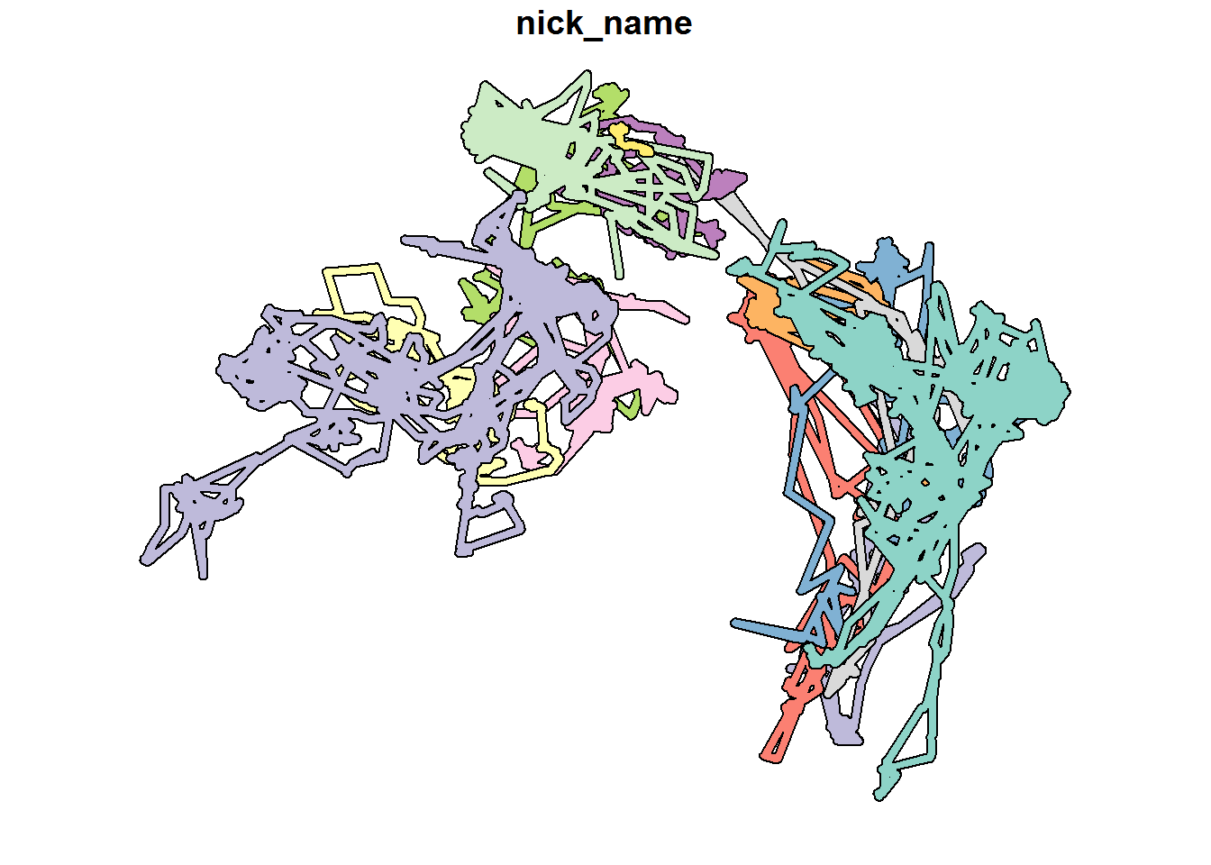
Here are the buffered locations superimposed on the EOSD, which we also crop somewhat to be more tight around the Hay River movement data (and save computation),
require(scales) # for alpha transparency
eosd <- crop(eosd, extent(hr.lines.buffered) %>% as.vector)
plot(eosd)
plot(eosd, add = TRUE, col = rgb(1,1,1,.3))
plot(hr.lines.buffered, add = TRUE)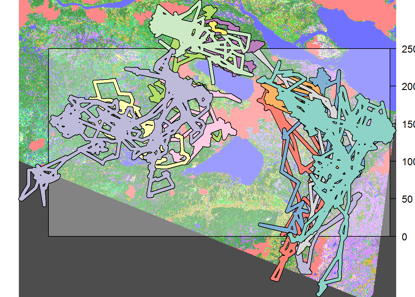
- Finally, in one fell swoop, you can mask the EOSD with all of these buffered lines. Note that we first combine all fo the lines into a single polygon:
hr.lines.buffered.combined <- st_union(hr.lines.buffered)
hr.eosd.buffered <- mask(eosd, as(hr.lines.buffered.combined, "Spatial"))Here’s the masked raster:
plot(hr.eosd.buffered)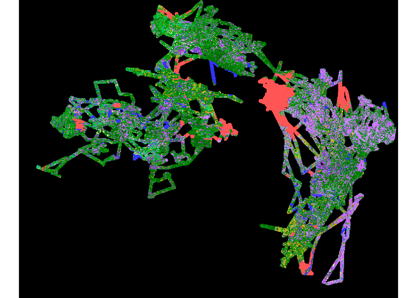
Computing a table of percentage coverage of the buffered location land class data:
hr.buffered.lc.table <- table(getValues(hr.eosd.buffered))
data.frame(Value = names(hr.buffered.lc.table),
Percentage = (prop.table(hr.buffered.lc.table)*100) %>% round(1) %>% as.numeric) %>%
merge(levels(eosd)[[1]][,c("Value", "Description")])## Value Percentage Description
## 1 100 0.0 Herbs
## 2 12 0.0 Shadow
## 3 20 4.3 Water
## 4 211 17.5 Coniferous-dense
## 5 212 29.8 Coniferous-open
## 6 213 5.4 Coniferous-sparse
## 7 221 0.2 Broadleaf-dense
## 8 222 0.3 Broadleaf-open
## 9 231 3.9 Mixedwood-dense
## 10 232 1.5 Mixedwood-open
## 11 250 7.8 Recent Burn
## 12 33 0.0 Exposed/Barren Land
## 13 34 0.2 Developed
## 14 40 0.1 Bryoids
## 15 51 0.1 Shrub Tall
## 16 52 0.6 Shrub Low
## 17 81 6.1 Wetland-treed
## 18 82 13.3 Wetland-shrub
## 19 83 6.1 Wetland-herb5 Putting it together: Location vs. Buffered vs. Available
A final barplot of values, following the example from the straight extraction at the top of this primer:
hr.lc.table <- table(raster::extract(eosd, st_coordinates(hayriver.sf)))
count.df <- data.frame(Value = names(hr.buffered.lc.table),
LC.buffered = hr.buffered.lc.table %>% as.numeric) %>%
merge(data.frame(Value = names(hr.lc.table), LC.location = hr.lc.table %>% as.numeric)) %>%
merge(levels(eosd)[[1]][,c("Value", "Description","Color","Count")])
count.df$p.Buffered <- prop.table(count.df$LC.buffered)
count.df$p.Location <- prop.table(count.df$LC.location)
count.df$p.Available <- prop.table(count.df$Count)
par(mar = c(3,10,2,2), cex.axis = 0.8, mgp = c(1, .1,0), tck = -.01)
with(arrange(count.df, p.Available),
barplot(rbind(p.Buffered, p.Location, p.Available),
horiz = TRUE, las = 1, beside = TRUE, bor = NA,
col = rbind(alpha(Color, 0.7), alpha(Color, 0.4), Color),
yaxt = "n", xlab = "proportion habitat used"))
mtext(side = 2, at = seq(0, 4*nrow(count.df) - 4, length = 14)+3,
text = arrange(count.df, p.Available)$Description, las = 1, cex = 0.7)
legend("bottomright", fill = rgb(0,0,0,c(1,0.2,0.6)),
legend = c("Available", "Location", "Buffered"), bty = "n")
axis(1)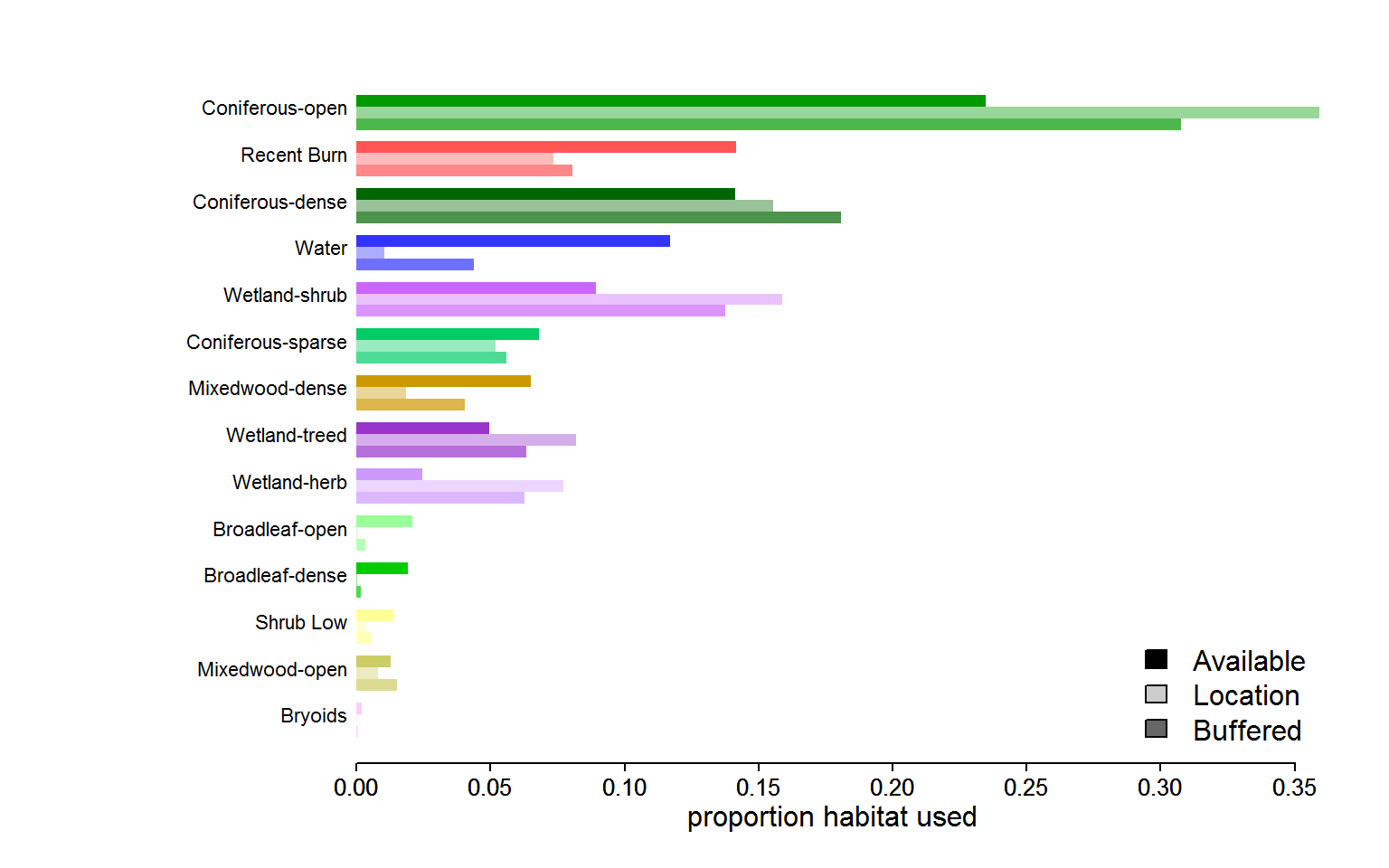
This is an interesting figure. It shows, in general, how strong the immediate selection of habitat can be, e.g. in the much stronger location based selection of “coniferous open” habitat, or the more obvious near absolute avoidance of water, though there is a considerable amount within a 1km radius (debatable, of course, whether water should ever be considered “avaialable”, esp in summer). Note also the “healthy distance” from dense broadleaf forest - not even in the 1km buffer is there much to be found.
6 Complete code
Click below to show complete code from this document.
knitr::opts_chunk$set(echo = TRUE, cache = TRUE, warning = FALSE, message = FALSE)
pcks <- c("move", "raster", "sf", "ggplot2", "plyr", "scales", "lubridate")
a <- sapply(pcks, require, character = TRUE)
## southies <- getMovebankData("ABoVE: NWT South Slave Boreal Woodland Caribou", login = mylogin)
## save(southies, file = "_data/southies.rda")
load("_data/southies.rda")
nrow(southies@idData)
southies.df <- as.data.frame(southies)
require(magrittr) # for piping
require(plyr) # for data frame manipulation
southies.timerange <- southies.df %>% ddply(c("nick_name","habitat"), summarize, start = min(timestamp), end = max(timestamp)) %>%
plyr::arrange(habitat,start) %>%
mutate(nick_name = as.factor(1:length(unique(nick_name))))
# this last line of code is just to make the ordering work right in the figure below
require(ggplot2)
ggplot(southies.timerange, aes(x = start, y = nick_name, col = habitat)) +
geom_segment(aes(x = start, xend = end, yend = nick_name)) + theme_bw()
ggplot(southies.df, aes(location_long, location_lat, col = habitat)) + geom_path() + theme_bw()
southies@proj4string
eosd <- raster("./_data/rasters/EOSD_withfire")
plot(eosd)
legend("topright", fill = levels(eosd)[[1]]$Color,
       legend = levels(eosd)[[1]]$Description, ncol = 2, cex = 0.55)
require(lubridate) # for the ymd function below
hayriver.sf <- southies.df %>% subset(habitat == "Hay River Lowlands" & timestamp < ymd("2012-01-01")) %>%
    st_as_sf(coords = c("location_long", "location_lat"), crs = projection(southies)) %>% st_transform(projection(eosd))
plot(eosd)
nick_names <- unique(hayriver.sf$nick_name)
greys <- grey(seq(.5,1,length = length(nick_names)))

for(i in 1:length(nick_names)){
    xy <- st_coordinates(subset(hayriver.sf, nick_name == nick_names[i]))
    lines(xy, col = greys[i])
}
crs(hayriver.sf)
crs(eosd)
## hayriver.landcover <- raster::extract(eosd, st_coordinates(hayriver.sf))
## save(hayriver.landcover, file = "./_data/hayriver_extract.rda")
load("./_data/hayriver_extract.rda")
table(hayriver.landcover)
levels(eosd)
hayriver.landclass <- with(levels(eosd)[[1]], Description[match(hayriver.landcover, Value)])
par(mar = c(3,10,2,2))
barplot(table(hayriver.landclass), horiz = TRUE, las = 1)
count.df <- data.frame(Description = names(table(hayriver.landclass)),
                       CaribouCount = table(hayriver.landclass) %>% as.numeric) %>% merge(
                         levels(eosd)[[1]][,c("Description","Color","Count")])

par(mar = c(3,10,2,2))
with(arrange(count.df, CaribouCount),
     barplot(CaribouCount, horiz = TRUE, las = 1, col = Color, names.arg = Description))
count.df$p.Used <- prop.table(count.df$CaribouCount)
count.df$p.Available <- prop.table(count.df$Count)

par(mar = c(3,10,2,2))
with(arrange(count.df, CaribouCount),
     barplot(rbind(p.Used, p.Available), horiz = TRUE, las = 1, beside = TRUE, bor = NA,
             col = rbind(alpha(Color, 0.5), Color),
             axes = FALSE))

mtext(side = 2, at = seq(3,60,3) - .5,
      text = arrange(count.df, CaribouCount)$Description, las = 1, cex = 0.7)
legend("bottomright", fill = c("black","grey"), legend = c("available", "used"), bty = "n")
extent(hayriver.sf[1,])
(crop.extent <- extent(hayriver.sf[1,]) + 2e3 * c(-1,1,-1,1))
eosd.cropped <- crop(eosd, crop.extent)
plot(eosd.cropped)
plot(st_geometry(hayriver.sf[1,]), col = "black", lwd = 2, cex = 3, pch = 21, bg = "white", add = TRUE)

xy <- st_coordinates(hayriver.sf[1,])[1,]
radius <- 1e3
z.circle <- (xy[1] + 1i*xy[2]) + complex(mod = radius, arg = seq(0, 2*pi, length = 1000))
circle.sf <- st_polygon(x = list(cbind(X = Re(z.circle), Y = Im(z.circle))))
plot(st_geometry(circle.sf), add = TRUE, col = rgb(1,1,1,.3))
require(raster); require(sf)
load("_data/southies.rda")
eosd <- raster("./_data/rasters/EOSD_withfire")
#hayriver.sf <- southies.df %>% subset(habitat == "Hay River Lowlands" & timestamp < ymd("2012-01-01")) %>%
# st_as_sf(coords = c("location_long", "location_lat"), crs = projection(southies)) %>% st_transform(projection(eosd))
raster::extract(eosd, hayriver.sf[1,], buffer = 1000, fun = function(x) which.max(tabulate(x)))
levels(eosd)
hr108 <- subset(hayriver.sf, nick_name == "HR108")
system.time(
  landcover.mode <- raster::extract(eosd, hr108, buffer = 1000, fun = function(x) which.max(tabulate(x)))
)
table(landcover.mode)
levels <- levels(eosd)[[1]]
hr108.levels <- levels[match(names(table(landcover.mode)), levels$Value),]
hr108.levels
barplot(table(landcover.mode), col = hr108.levels$Color,
        legend.text = hr108.levels$Description, args.legend=list(x = "topleft"))
eosd.masked <- mask(eosd.cropped, as(circle.sf, "Spatial"))
plot(eosd.masked)
table(getValues(eosd.masked))
getLandcoverInBuffer <- function(xy, radius){
  xy <- st_coordinates(xy)[1,]
  crop.extent <- xy + radius * c(-1,1,-1,1)
  eosd.cropped <- crop(eosd, crop.extent)
  z.circle <- (xy[1] + 1i*xy[2]) + complex(mod = radius, arg = seq(0, 2*pi, length = 1000))
  circle.sf <- st_polygon(x = list(cbind(X = Re(z.circle), Y = Im(z.circle))))
  eosd.masked <- mask(eosd.cropped, as(circle.sf, "Spatial"))
  table(getValues(eosd.masked))
}

getLandcoverInBuffer(hayriver.sf[1,], 1e3)
getLandcoverInBuffer(hayriver.sf[5,], 1e3)
system.time(getLandcoverInBuffer(hayriver.sf[1,], 1e3))
hr108 <- subset(hayriver.sf, nick_name == "HR108")[1:30,]
## # initialize matrix with 250(!) columns for each possible value to populate with results of the table count
## landcover.matrix <- matrix(NA, nrow = nrow(hr108), ncol = 250)
## system.time(
## for(i in 1:nrow(hr108)){
## my.lcs <- getLandcoverInBuffer(hayriver.sf[i,], 1e3)
## which <- as.numeric(names(my.lcs))
## landcover.matrix[i,which] <- as.numeric(my.lcs)
## })
load("_data/landcover.matrix.rda")
# apply runs a function across dimensions (in this case 1 = rows) of a matrix  ... unfortunately it also turns it sideways (in this case), hence the `t` at the end
p.landcover.matrix <- apply(landcover.matrix, 1, function(x) x/(sum(x, na.rm = TRUE))) %>% t
# change the NA's to 0's
p.landcover.matrix[is.na(p.landcover.matrix)] <- 0
data_columns <- colSums(p.landcover.matrix) > 0
p.landcover.df <- data.frame(p.landcover.matrix[,data_columns])
names(p.landcover.df) <- which(data_columns)
head(p.landcover.df)
par(bty="l", mgp = c(1.5,.25,0), tck = 0.01)
levels <- levels(eosd)[[1]]
legend.table <- levels[match(names(p.landcover.df), levels$Value), ]

matplot(hr108$timestamp,  p.landcover.df, type="o", pch = 19, lty = 1,
        col = legend.table$Color, lwd = 1, xlab = "time", xaxt="n", ylim = c(0,1))
# some non-intuitive code to make the x-axis show times correctly
axis(1, at = pretty(hr108$timestamp), labels = as.character(pretty(hr108$timestamp)))
legend("top", col = legend.table$Color, pch = 19, lty = 1, legend = legend.table$Description, ncol = 3, cex = 0.8, bty = "n")
par(bty="l", mgp = c(1.5,.25,0), tck = 0.01, cex.axis = 0.8, las = 1)
time <- hr108$timestamp
ddays <- difftime(time[-1], time[-nrow(hr108)], units = "days") %>% as.numeric

barplot(p.landcover.df %>% t %>% as.matrix, space = 0,
        width = c(0,ddays),
        col = legend.table$Color, bor = NA, sep = 0)
totaltime <- difftime(max(time), min(time), units= "days")

axis(1, at = difftime(pretty(time,  n = 10), min(time), units = "days"),
     labels = as.character(pretty(time,  n = 10)))
## save(p.landcover2.df, eosd.levels, hr108.levels, file = "_data/p.landcover2.df.rda")
load(file = "_data/p.landcover2.df.rda")
hr108 <- subset(hayriver.sf, nick_name == nick_name[1])
eosd.values <- levels(eosd)[[1]]$Value
system.time(
  landcover2.matrix <- sapply(eosd.values,
                              function(v) raster::extract(eosd, hr108, buffer = 1e3, fun = function(x) sum(x == v)))
)
colnames(landcover2.matrix) <- eosd.values
p.landcover2.df <- apply(landcover2.matrix, 1, function(x) x/(sum(x, na.rm = TRUE))) %>% t %>% as.data.frame
time <- hr108$timestamp
ddays <- difftime(time[-1], time[-nrow(hr108)], units = "days") %>% as.numeric
eosd.levels <- levels(eosd)[[1]]
hr108.levels <- eosd.levels[match(names(p.landcover2.df), eosd.levels$Value),]
par(bty="l", mgp = c(1.5,.25,0), tck = 0.01, cex.axis = 0.8, las = 1, mar = c(3,3,2,2))
load(file = "_data/p.landcover2.df.rda")
barplot(p.landcover2.df %>% t %>% as.matrix, space = 0,
        width = c(0,ddays),  legend.text = hr108.levels$Description, args.legend=list(cex = 0.7, bty = "n"),
        col = hr108.levels$Color, bor = NA, sep = 0,
        xlim = c(0,sum(ddays)*1.3))
totaltime <- difftime(max(time), min(time), units= "days")

axis(1, at = difftime(pretty(time,  n = 10), min(time), units = "days"),
     labels = as.character(pretty(time,  n = 10)))
# key package (though there are others)
library(parallel)
# generate the cluster.   THe 4 is the number of cores on my laptop, but I have, e.g., 8 on my desktop, for example.
cl = makeCluster(4)
# important for all the cores to have access to the raster, the movement data, and the raster package:
clusterExport(cl, list('eosd','hr108'))
clusterEvalQ(cl, library(raster))
# do a parallel sapply:
system.time(
  hr2 <- parSapply(cl, eosd.values,
                   function(v) raster::extract(eosd, hr108, buffer = 1e3,
                                                fun = function(x) sum(x == v)))
)
#setwd("C:/Users/Elie/Box Sync/caribou/NWT/rsf/primers")
pcks <- c("raster", "sf", "ggplot2", "plyr", "scales", "lubridate", "magrittr")
a <- sapply(pcks, require, character = TRUE)
load("_data/southies.rda")
eosd <- raster("./_data/rasters/EOSD_withfire")
southies.df <- as.data.frame(southies)
hayriver.sf <- southies.df %>% subset(habitat == "Hay River Lowlands" & timestamp < ymd("2012-01-01")) %>%
st_as_sf(coords = c("location_long", "location_lat"), crs = projection(southies)) %>% st_transform(projection(eosd))
require(dplyr)
hayriver.lines <- hayriver.sf[,c("habitat","nick_name")] %>% group_by(nick_name) %>%
  summarize(do_union=FALSE) %>% st_cast("LINESTRING") %>% st_transform(projection(eosd))
hayriver.lines
hr.lines.buffered <- st_buffer(hayriver.lines, 1e3)
plot(hr.lines.buffered)
require(scales)  # for alpha transparency
eosd <- crop(eosd, extent(hr.lines.buffered) %>% as.vector)
plot(eosd)
plot(eosd, add = TRUE, col = rgb(1,1,1,.3))
plot(hr.lines.buffered, add = TRUE)
hr.lines.buffered.combined <- st_union(hr.lines.buffered)
hr.eosd.buffered <- mask(eosd, as(hr.lines.buffered.combined, "Spatial"))
plot(hr.eosd.buffered)
hr.buffered.lc.table <- table(getValues(hr.eosd.buffered))

data.frame(Value = names(hr.buffered.lc.table),
           Percentage  = (prop.table(hr.buffered.lc.table)*100) %>% round(1) %>% as.numeric) %>%
  merge(levels(eosd)[[1]][,c("Value", "Description")])
hr.lc.table <- table(raster::extract(eosd, st_coordinates(hayriver.sf)))
count.df <- data.frame(Value = names(hr.buffered.lc.table),
                       LC.buffered = hr.buffered.lc.table %>% as.numeric) %>%
  merge(data.frame(Value = names(hr.lc.table), LC.location = hr.lc.table %>% as.numeric)) %>%
  merge(levels(eosd)[[1]][,c("Value", "Description","Color","Count")])

count.df$p.Buffered <- prop.table(count.df$LC.buffered)
count.df$p.Location <- prop.table(count.df$LC.location)
count.df$p.Available <- prop.table(count.df$Count)

par(mar = c(3,10,2,2), cex.axis = 0.8, mgp = c(1, .1,0), tck = -.01)
with(arrange(count.df, p.Available),
     barplot(rbind(p.Buffered, p.Location, p.Available),
             horiz = TRUE, las = 1, beside = TRUE, bor = NA,
             col = rbind(alpha(Color, 0.7), alpha(Color, 0.4), Color),
             yaxt = "n", xlab = "proportion habitat used"))
mtext(side = 2, at = seq(0, 4*nrow(count.df) - 4, length = 14)+3,
      text = arrange(count.df, p.Available)$Description, las = 1, cex = 0.7)
legend("bottomright", fill = rgb(0,0,0,c(1,0.2,0.6)),
       legend = c("Available", "Location", "Buffered"), bty = "n")
axis(1)