Loading EOSD rasters and updating with fire polygons
Elie Gurarie and Laura Berman
UPDATED: 2019-09-27
Goals:
- Load, process and summarize EOSD Canadian forest land cover raster data
- Add layer desciptions (from external file) to existing EOSD raster
- Load Fire polygon data, visualize, convert to raster
- Reclassify EOSD raster with fires
List of required packages for these tasks (the code below will load all of them):
pcks <- c("raster", "sf", "ggplot2", "plyr", "scales")
sapply(pcks, require, character = TRUE)
## raster sf ggplot2 plyr scales
## TRUE TRUE TRUE TRUE TRUE1 Land cover raster
1.1 Loading the raster
require(raster)The Raster package is capable of loading all kinds of rasterized data formats, including geotiffs (one of the more common and compact formats). It’s an important package to have installed if you are working with raster objects.
We are working with an EOSD (Earth Observation for Sustainable Development of Forests) raster object. EOSD is a land cover map of the forested area of Canada. We will be working with just one clip (one section of the map).
The complete set of EOSD data files we will be using can be found here:
list.files("./_data/EOSD")## [1] "EOSD Legend.docx" "EOSD_FMDColours.lyr"
## [3] "EOSD_legend.txt" "EOSD_NWT_HRL_clip.tfw"
## [5] "EOSD_NWT_HRL_clip.tif" "EOSD_NWT_HRL_clip.tif.aux.xml"
## [7] "EOSD_NWT_HRL_clip.tif.ovr" "EOSD_NWT_HRL_clip.tif.vat.cpg"
## [9] "EOSD_NWT_HRL_clip.tif.vat.dbf" "EOSD_NWT_HRL_clip.tif.xml"
## [11] "EOSD_README.txt" "legend.TIF"As you can tell from the command above, the EOSD data is in a folder called: ./_data/EOSD (because that’s where we put it). This clip is from the Hay River lowlands, and you’ll note that (most of) these files start with EOST_NWT_HRL_clip. We load the tif file with the raster command:
EOSD <- raster("./_data/EOSD/EOSD_NWT_HRL_clip.tif")Even though the raster is huuuuuuge, this loads quickly and “silently”. There are no error messages. The reason is that the data is not actually in R’s memory - the raster command is an instruction to know where to look for the data as needed.
1.2 Plot the raster
Use the plot function to plot the raster object that was defined in the previous line of code:
plot(EOSD)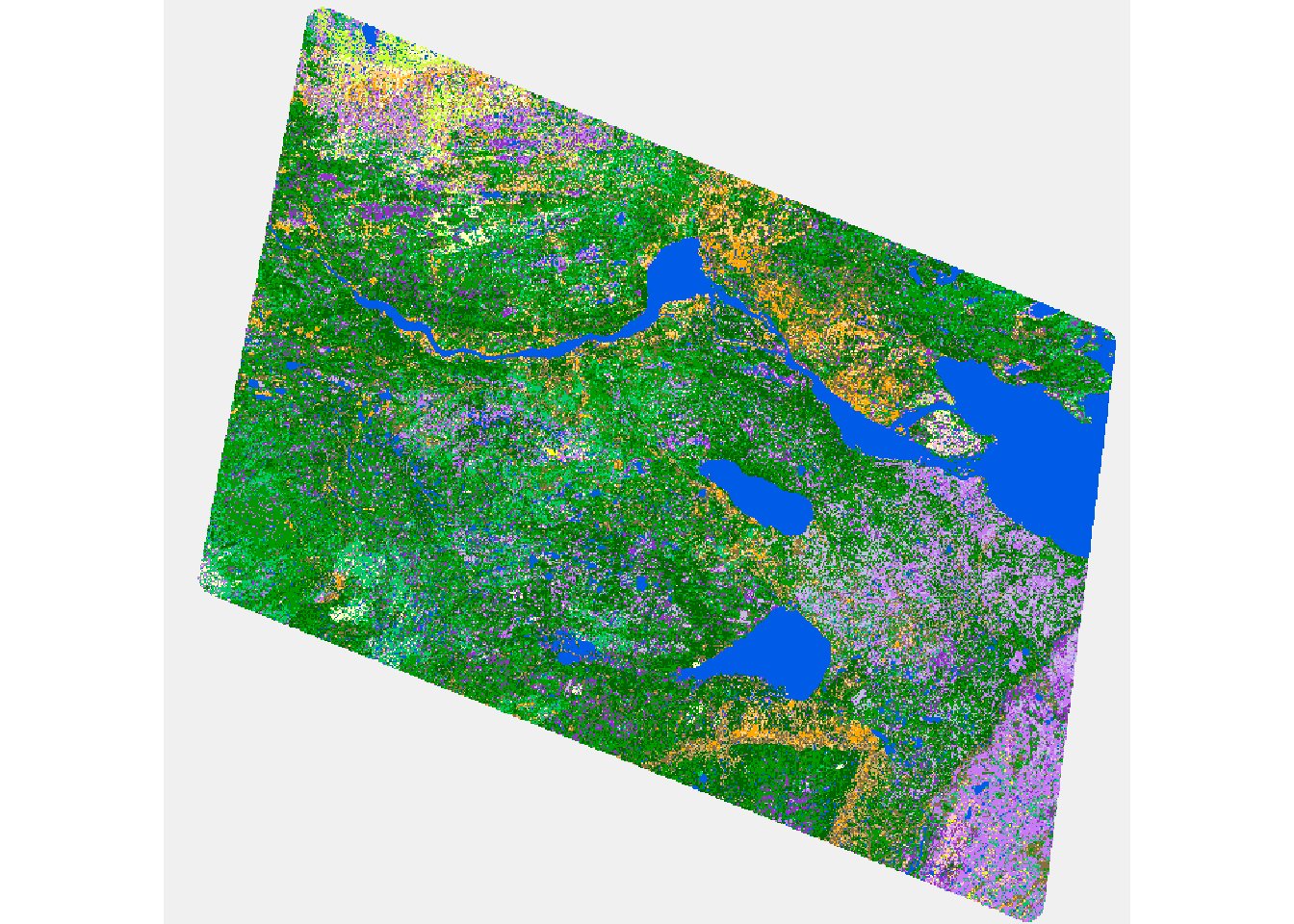
1.3 Structure of the raster object
If you type in EOSD, you get some useful basic information:
EOSD## class : RasterLayer
## dimensions : 8895, 9305, 82767975 (nrow, ncol, ncell)
## resolution : 30, 30 (x, y)
## extent : -475896.4, -196746.4, 2214172, 2481022 (xmin, xmax, ymin, ymax)
## coord. ref. : +proj=aea +lat_1=50 +lat_2=70 +lat_0=40 +lon_0=-112 +x_0=0 +y_0=0 +datum=NAD83 +units=m +no_defs +ellps=GRS80 +towgs84=0,0,0
## data source : C:/Users/Elie/Box Sync/caribou/NWT/rsf/primers/_data/EOSD/EOSD_NWT_HRL_clip.tif
## names : EOSD_NWT_HRL_clip
## values : 12, 232 (min, max)
## attributes :
## ID OBJECTID Value Count
## from: 0 1 12 366
## to : 18 19 232 682104AS with the movestack object in the Primer 1, this is a complex S4 object with lots of buried information. You can reveal this buried information by using the str() command (or, in newer versions of Rstudio, interactively by clicking on EOSD in the environment window):
str(EOSD)## Formal class 'RasterLayer' [package "raster"] with 12 slots
## ..@ file :Formal class '.RasterFile' [package "raster"] with 13 slots
## .. .. ..@ name : chr "C:\\Users\\Elie\\Box Sync\\caribou\\NWT\\rsf\\primers\\_data\\EOSD\\EOSD_NWT_HRL_clip.tif"
## .. .. ..@ datanotation: chr "INT1U"
## .. .. ..@ byteorder : chr "little"
## .. .. ..@ nodatavalue : num -Inf
## .. .. ..@ NAchanged : logi FALSE
## .. .. ..@ nbands : int 1
## .. .. ..@ bandorder : chr "BIL"
## .. .. ..@ offset : int 0
## .. .. ..@ toptobottom : logi TRUE
## .. .. ..@ blockrows : int 128
## .. .. ..@ blockcols : int 128
## .. .. ..@ driver : chr "gdal"
## .. .. ..@ open : logi FALSE
## ..@ data :Formal class '.SingleLayerData' [package "raster"] with 13 slots
## .. .. ..@ values : logi(0)
## .. .. ..@ offset : num 0
## .. .. ..@ gain : num 1
## .. .. ..@ inmemory : logi FALSE
## .. .. ..@ fromdisk : logi TRUE
## .. .. ..@ isfactor : logi TRUE
## .. .. ..@ attributes:List of 1
## .. .. .. ..$ :'data.frame': 19 obs. of 4 variables:
## .. .. .. .. ..$ ID : int [1:19] 0 1 2 3 4 5 6 7 8 9 ...
## .. .. .. .. ..$ OBJECTID: int [1:19] 1 2 3 4 5 6 7 8 9 10 ...
## .. .. .. .. ..$ Value : int [1:19] 12 20 32 33 34 40 51 52 81 82 ...
## .. .. .. .. ..$ Count : num [1:19] 366 5813291 77 15049 68107 ...
## .. .. ..@ haveminmax: logi TRUE
## .. .. ..@ min : num 12
## .. .. ..@ max : num 232
## .. .. ..@ band : int 1
## .. .. ..@ unit : chr ""
## .. .. ..@ names : chr "EOSD_NWT_HRL_clip"
## ..@ legend :Formal class '.RasterLegend' [package "raster"] with 5 slots
## .. .. ..@ type : chr(0)
## .. .. ..@ values : logi(0)
## .. .. ..@ color : logi(0)
## .. .. ..@ names : logi(0)
## .. .. ..@ colortable: chr [1:256] "#F0F0F0" "#000000" "#000000" "#000000" ...
## ..@ title : chr(0)
## ..@ extent :Formal class 'Extent' [package "raster"] with 4 slots
## .. .. ..@ xmin: num -475896
## .. .. ..@ xmax: num -196746
## .. .. ..@ ymin: num 2214172
## .. .. ..@ ymax: num 2481022
## ..@ rotated : logi FALSE
## ..@ rotation:Formal class '.Rotation' [package "raster"] with 2 slots
## .. .. ..@ geotrans: num(0)
## .. .. ..@ transfun:function ()
## ..@ ncols : int 9305
## ..@ nrows : int 8895
## ..@ crs :Formal class 'CRS' [package "sp"] with 1 slot
## .. .. ..@ projargs: chr "+proj=aea +lat_1=50 +lat_2=70 +lat_0=40 +lon_0=-112 +x_0=0 +y_0=0 +datum=NAD83 +units=m +no_defs +ellps=GRS80 +towgs84=0,0,0"
## ..@ history : list()
## ..@ z : list()str() reveals the structure of the raster object. Here you can see all of the slots within the raster, and each of the slots nested within those slots.
Again, one useful slot is the projection. Here are two different ways of showing the projection:
EOSD@crs## CRS arguments:
## +proj=aea +lat_1=50 +lat_2=70 +lat_0=40 +lon_0=-112 +x_0=0 +y_0=0
## +datum=NAD83 +units=m +no_defs +ellps=GRS80 +towgs84=0,0,0projection(EOSD)## [1] "+proj=aea +lat_1=50 +lat_2=70 +lat_0=40 +lon_0=-112 +x_0=0 +y_0=0 +datum=NAD83 +units=m +no_defs +ellps=GRS80 +towgs84=0,0,0"EOSD@crs displays the crs(coordinate reference system) slot of the EOSD raster layer. The projection function is used to display the coordinate reference system of a raster object. Both of these functions will give you the same information.
This is an Albers Equal Area projection, useful for northern latitudes and presumably the projection used for the complete NWT_EOSD data set.
Now, here are two ways to see the extent of the data (a different slot in the raster):
EOSD@extent## class : Extent
## xmin : -475896.4
## xmax : -196746.4
## ymin : 2214172
## ymax : 2481022bbox(EOSD)## min max
## s1 -475896.4 -196746.4
## s2 2214172.2 2481022.2EOSD@extent works the same way that EOSD@crs did. It displays one particular slot in the raster layer, in this case the extent slot. The bbox function is specifically used to retreive the spatial bounding box from spatial data, hence the name: bbox = bounding box.
These two functions will give you the same information, but in slightly different formats. EOSD@extent is a little more user-friendly to read. Just note that “s1” is the same as “x” and “s2” is the same as “y”.
You can also use the “@” command to look specifically at the slots within certain slots:
EOSD@data@attributes[[1]]## ID OBJECTID Value Count
## 1 0 1 12 366
## 2 1 2 20 5813291
## 3 2 3 32 77
## 4 3 4 33 15049
## 5 4 5 34 68107
## 6 5 6 40 104911
## 7 6 7 51 75701
## 8 7 8 52 808924
## 9 8 9 81 2822861
## 10 9 10 82 4762600
## 11 10 11 83 1445821
## 12 11 12 100 571282
## 13 12 13 211 8013451
## 14 13 14 212 13630642
## 15 14 15 213 3797694
## 16 15 16 221 991126
## 17 16 17 222 1096492
## 18 17 18 231 3489275
## 19 18 19 232 682104If you look back up at str(EOSD) you’ll see that attributes is one of 13 slots within data, which is a slot within EOSD. You can use this same command to look at any part of the raster. THis info is also obtained via:
levels(EOSD)[[1]]## ID OBJECTID Value Count
## 1 0 1 12 366
## 2 1 2 20 5813291
## 3 2 3 32 77
## 4 3 4 33 15049
## 5 4 5 34 68107
## 6 5 6 40 104911
## 7 6 7 51 75701
## 8 7 8 52 808924
## 9 8 9 81 2822861
## 10 9 10 82 4762600
## 11 10 11 83 1445821
## 12 11 12 100 571282
## 13 12 13 211 8013451
## 14 13 14 212 13630642
## 15 14 15 213 3797694
## 16 15 16 221 991126
## 17 16 17 222 1096492
## 18 17 18 231 3489275
## 19 18 19 232 682104I’m not sure why the levels is list, but it is, and we need the first element (hence: [[1]]).
1.4 Updating the legend
Unfortunately, the EOSD data levels don’t have the classification names (or colors DIRECTLY associated with them). These exist in a different file (provided by James):
(EOSD.legend <- read.delim("./_data/EOSD/EOSD_legend.txt", sep = "\t"))## ID Value Description RGB.Code
## 1 1 0 No Data 0;0;0
## 2 2 11 Cloud 255;255;254
## 3 3 12 Shadow 51;51;51
## 4 4 20 Water 51;51;255
## 5 5 22 Canada Text 35;31;32
## 6 6 30 Non-Vegetated Land 153;102;102
## 7 7 31 Snow/Ice 204;255;255
## 8 8 32 Rock/Rubble 204;204;204
## 9 9 33 Exposed/Barren Land 153;102;51
## 10 10 34 Developed 204;102;153
## 11 11 40 Bryoids 255;204;255
## 12 12 44 Canada Flag 237;28;36
## 13 13 50 Shrubland 255;255;0
## 14 14 51 Shrub Tall 255;255;51
## 15 15 52 Shrub Low 255;255;153
## 16 16 80 Wetland 153;51;153
## 17 17 81 Wetland-treed 153;51;204
## 18 18 82 Wetland-shrub 204;102;255
## 19 19 83 Wetland-herb 204;153;255
## 20 20 100 Herbs 204;255;51
## 21 21 110 Grassland 204;204;0
## 22 22 120 Agriculture 204;102;0
## 23 23 121 Agr-Cropland 255;153;51
## 24 24 122 Agr-Pasture/Forage 255;204;51
## 25 25 200 Forest/Trees 0;153;0
## 26 26 210 Coniferous 0;102;0
## 27 27 211 Coniferous-dense 0;102;0
## 28 28 212 Coniferous-open 0;153;0
## 29 29 213 Coniferous-sparse 0;204;102
## 30 30 220 Broadleaf 0;204;0
## 31 31 221 Broadleaf-dense 0;204;0
## 32 32 222 Broadleaf-open 153;255;153
## 33 33 223 Broadleaf-sparse 204;255;153
## 34 34 230 Mixedwood 204;153;0
## 35 35 231 Mixedwood-dense 204;153;0
## 36 36 232 Mixedwood-open 204;204;102
## 37 37 233 Mixedwood-sparse 204;204;153A bit of an issue with the RGB.Code to convert that to something R understands (check out this trick here: https://stackoverflow.com/questions/31574480/rgb-to-hex-converter).
RGB.raw <- as.character(EOSD.legend$RGB.Code)
Colors <- sapply(strsplit(RGB.raw, ";"), function(x) rgb(x[1], x[2], x[3], maxColorValue = 255))
EOSD.legend$Color <- Colors
Now, we can replace the “levels” of the original EOSD with this data frame, and use it as a basis for plotting later. We have to be a bit careful because the number of levels doesn’t quite match up (19 vs. 37):
str(levels(EOSD)[[1]])## 'data.frame': 19 obs. of 4 variables:
## $ ID : int 0 1 2 3 4 5 6 7 8 9 ...
## $ OBJECTID: int 1 2 3 4 5 6 7 8 9 10 ...
## $ Value : int 12 20 32 33 34 40 51 52 81 82 ...
## $ Count : num 366 5813291 77 15049 68107 ...str(EOSD.legend)## 'data.frame': 37 obs. of 5 variables:
## $ ID : int 1 2 3 4 5 6 7 8 9 10 ...
## $ Value : int 0 11 12 20 22 30 31 32 33 34 ...
## $ Description: Factor w/ 37 levels "Agr-Cropland",..: 25 11 28 33 10 26 32 27 17 16 ...
## $ RGB.Code : Factor w/ 33 levels "0;0;0","0;102;0",..: 1 29 33 32 31 6 21 19 7 12 ...
## $ Color : chr "#000000" "#FFFFFE" "#333333" "#3333FF" ...So we need to “merge” the two data frames using “Value” as the link and retain only the rows in the original levels.
(LevelsMerged <- merge(levels(EOSD)[[1]], EOSD.legend[,c("Value","Description","Color")], by = "Value", all.x = TRUE))## Value ID OBJECTID Count Description Color
## 1 12 0 1 366 Shadow #333333
## 2 20 1 2 5813291 Water #3333FF
## 3 32 2 3 77 Rock/Rubble #CCCCCC
## 4 33 3 4 15049 Exposed/Barren Land #996633
## 5 34 4 5 68107 Developed #CC6699
## 6 40 5 6 104911 Bryoids #FFCCFF
## 7 51 6 7 75701 Shrub Tall #FFFF33
## 8 52 7 8 808924 Shrub Low #FFFF99
## 9 81 8 9 2822861 Wetland-treed #9933CC
## 10 82 9 10 4762600 Wetland-shrub #CC66FF
## 11 83 10 11 1445821 Wetland-herb #CC99FF
## 12 100 11 12 571282 Herbs #CCFF33
## 13 211 12 13 8013451 Coniferous-dense #006600
## 14 212 13 14 13630642 Coniferous-open #009900
## 15 213 14 15 3797694 Coniferous-sparse #00CC66
## 16 221 15 16 991126 Broadleaf-dense #00CC00
## 17 222 16 17 1096492 Broadleaf-open #99FF99
## 18 231 17 18 3489275 Mixedwood-dense #CC9900
## 19 232 18 19 682104 Mixedwood-open #CCCC66We NEED to have ID be the first column ….
LevelsMerged <- LevelsMerged[,c("ID","OBJECTID","Value","Description","Color","Count")]We can now replace the ID in the EOSD.
levels(EOSD)[[1]] <- LevelsMergedTo be VERY VERY careful about these kinds of changes, we need to also undertand how raster color codes its images. If there are no colors provided, it will look inside a slot inside a slot called @legend@colortable:
EOSD@legend@colortable## [1] "#F0F0F0" "#000000" "#000000" "#000000" "#000000" "#000000" "#000000"
## [8] "#000000" "#000000" "#000000" "#000000" "#FFFFFF" "#4E4E4E" "#000000"
## [15] "#000000" "#000000" "#000000" "#000000" "#000000" "#000000" "#005CE6"
## [22] "#000000" "#000000" "#000000" "#000000" "#000000" "#000000" "#000000"
## [29] "#000000" "#000000" "#000000" "#CAFDFD" "#CACACA" "#976430" "#976430"
## [36] "#000000" "#000000" "#000000" "#000000" "#000000" "#FFBEE8" "#000000"
## [43] "#000000" "#000000" "#000000" "#000000" "#000000" "#000000" "#000000"
## [50] "#000000" "#000000" "#FFFF00" "#FFFFBE" "#000000" "#000000" "#000000"
## [57] "#000000" "#000000" "#000000" "#000000" "#000000" "#000000" "#000000"
## [64] "#000000" "#000000" "#000000" "#000000" "#000000" "#000000" "#000000"
## [71] "#000000" "#000000" "#000000" "#000000" "#000000" "#000000" "#000000"
## [78] "#000000" "#000000" "#000000" "#000000" "#9730CA" "#CA7AF5" "#C7BAE5"
## [85] "#000000" "#000000" "#000000" "#000000" "#000000" "#000000" "#000000"
## [92] "#000000" "#000000" "#000000" "#000000" "#000000" "#000000" "#000000"
## [99] "#000000" "#000000" "#CAFD30" "#000000" "#000000" "#000000" "#000000"
## [106] "#000000" "#000000" "#000000" "#000000" "#000000" "#000000" "#000000"
## [113] "#000000" "#000000" "#000000" "#000000" "#000000" "#000000" "#000000"
## [120] "#000000" "#000000" "#000000" "#000000" "#000000" "#000000" "#000000"
## [127] "#000000" "#000000" "#000000" "#000000" "#000000" "#000000" "#000000"
## [134] "#000000" "#000000" "#000000" "#000000" "#000000" "#000000" "#000000"
## [141] "#000000" "#000000" "#000000" "#000000" "#000000" "#000000" "#000000"
## [148] "#000000" "#000000" "#000000" "#000000" "#000000" "#000000" "#000000"
## [155] "#000000" "#000000" "#000000" "#000000" "#000000" "#000000" "#000000"
## [162] "#000000" "#000000" "#000000" "#000000" "#000000" "#000000" "#000000"
## [169] "#000000" "#000000" "#000000" "#000000" "#000000" "#000000" "#000000"
## [176] "#000000" "#000000" "#000000" "#000000" "#000000" "#000000" "#000000"
## [183] "#000000" "#000000" "#000000" "#000000" "#000000" "#000000" "#000000"
## [190] "#000000" "#000000" "#000000" "#000000" "#000000" "#000000" "#000000"
## [197] "#000000" "#000000" "#000000" "#000000" "#000000" "#000000" "#000000"
## [204] "#000000" "#000000" "#000000" "#000000" "#000000" "#000000" "#000000"
## [211] "#000000" "#006500" "#009700" "#00CA64" "#000000" "#000000" "#000000"
## [218] "#000000" "#000000" "#000000" "#000000" "#FFAA00" "#FFD37F" "#000000"
## [225] "#000000" "#000000" "#000000" "#000000" "#000000" "#000000" "#000000"
## [232] "#897044" "#CDAD66" "#000000" "#000000" "#000000" "#000000" "#000000"
## [239] "#000000" "#000000" "#000000" "#000000" "#000000" "#000000" "#000000"
## [246] "#000000" "#000000" "#000000" "#000000" "#000000" "#000000" "#000000"
## [253] "#000000" "#000000" "#000000" "#000000"These colors correspond to all the possible codes from 1 to 255 … here’s a visualization of these colors (that aren’t black: #000000).
which.not.black <- which(EOSD@legend@colortable != "#000000")
cols.not.black <- EOSD@legend@colortable[which.not.black]
plot(1:length(cols.not.black), bg = cols.not.black, pch = 21, cex = 3, bty = "l", axes = FALSE, xlab = "", ylab = "")
text(1:length(which.not.black), 1:length(which.not.black), which.not.black, font = 2, cex = 0.8)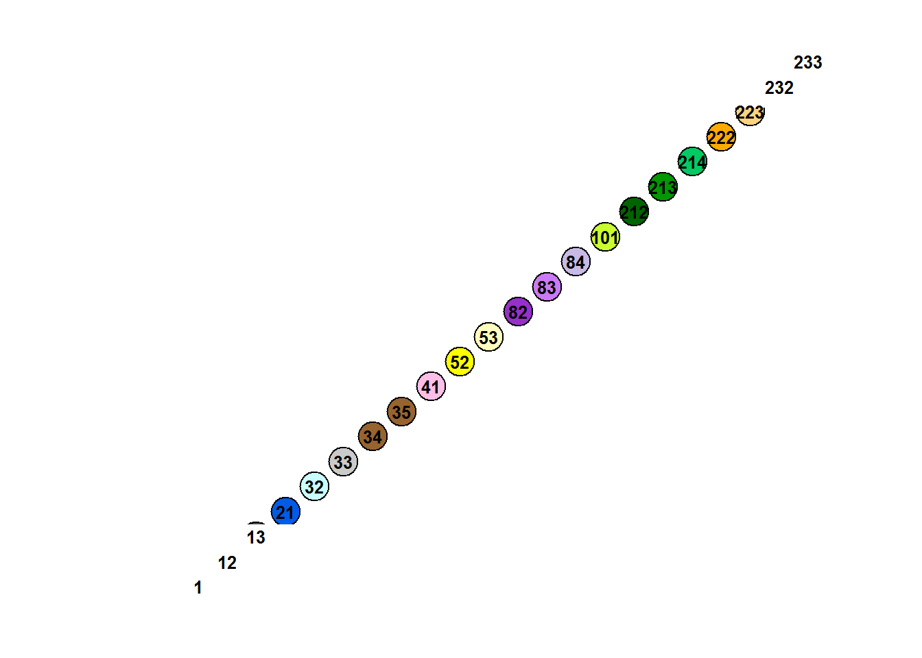
We should match the right colors to the right levels, but there’s an annoying trick where the numbering has to be from 0 not 1! We’ll do this for a small section of the data to see clearly what’s happening:
Cropped Data:
EOSD.crop <- crop(EOSD, extent(-411594.5, -384535.5, 2396389, 2419998))
plot(EOSD.crop)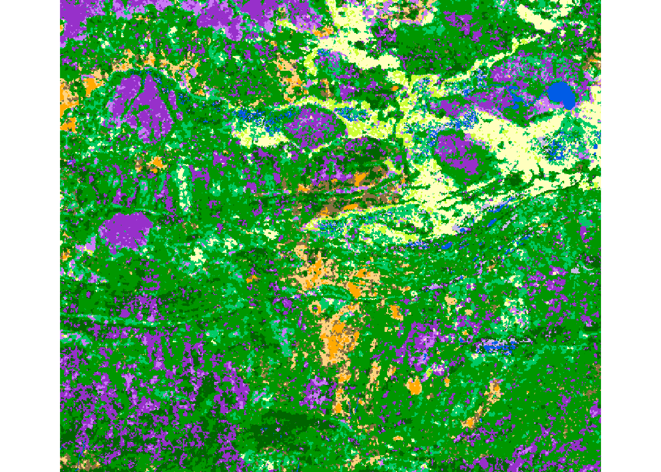
Replace the colors: We use the colors in the EOSD.legend and place them in the Values slot + 1.
EOSD.crop2 <- EOSD.crop
EOSD.crop2@legend@colortable[EOSD.legend$Value+1] <- EOSD.legend$Color
plot(EOSD.crop2)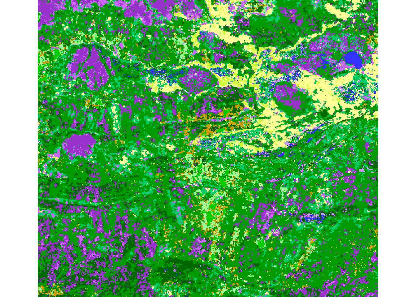
There are some subtle - but important differences (less orange - sad to see it go!). The plotting colors, however, WILL MATCH with the legend colors. So we’ll make this dramatic change:
EOSD@legend@colortable[EOSD.legend$Value+1] <- EOSD.legend$ColorAt this stage, it is a good idea to SAVE the revised EOSD object:
writeRaster(EOSD, file = "./_data/rasters/EOSD_updated.tif")The .tif format is the most space effective, and portable (i.e. can be opened sometimes just with an image viewer, and also ArcGIS and similar tools). UNFORTUNATELY, saving as a tiff will lose the attributes data and we can’t figure out what format to save it in to retain those data. However, to see how to add attributes to a .tif within ArcGIS, see: Step02b_ExportingRastersToArcGIS.html.
In the meantime, we will save rasters using R’s native format, which has extension grd:
writeRaster(EOSD, file = "./_data/rasters/EOSD_updated")1.5 Plotting and labeling with the new labels
Now that the data is “correct”, we can plot and provide a legend using our factor levels:
plot(EOSD, main = "EOSD in the Hay River Lowlands Clip")
legend("topright", fill = levels(EOSD)[[1]]$Color, legend = levels(EOSD)[[1]]$Description, ncol = 2, cex = 0.55)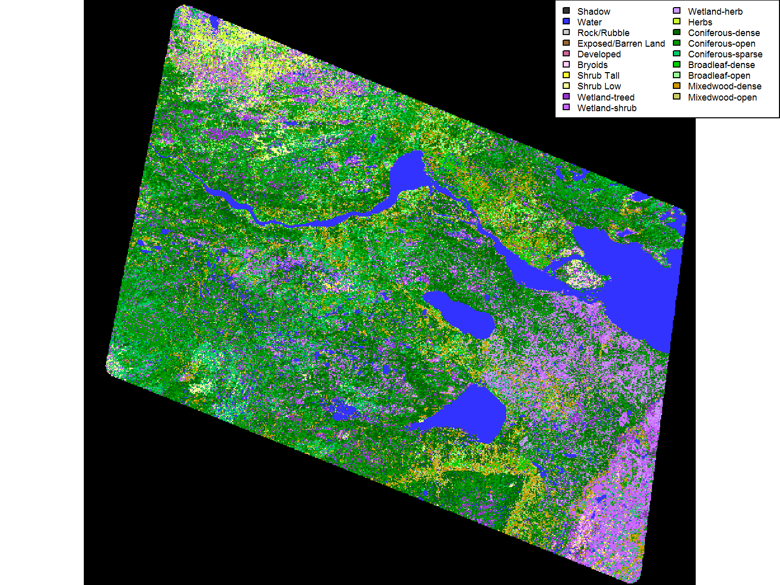
Note that the borders are now black (and there’s less orange). But at least we know what the colors corresoind to. Lots of wetland shrub, lots of different forest types.
The following code will compute the relative amount of each type, and make a bar plot. Note, we counted these from scratch, but they correspond to the counts that were already in the levels of the raster. Note, that this can take a little while for a large raster (which our EOSD clip already is).
counts <- table(getValues(EOSD))
counts
##
## 12 20 32 33 34 40 51 52
## 366 5813291 77 15049 68107 104911 75701 808924
## 81 82 83 100 211 212 213 221
## 2822861 4762600 1445821 571282 8013451 13630642 3797694 991126
## 222 231 232
## 1096492 3489275 682104counts.df <- cbind(levels(EOSD)[[1]], Count2 = as.vector(counts))And draw a barplot:
par(mar = c(4,10,2,2), cex = 0.8)
with(counts.df,
     barplot(Count, col = Color, names = Description,
        horiz = TRUE, las = 1, bor = NA,  main = "landcover"))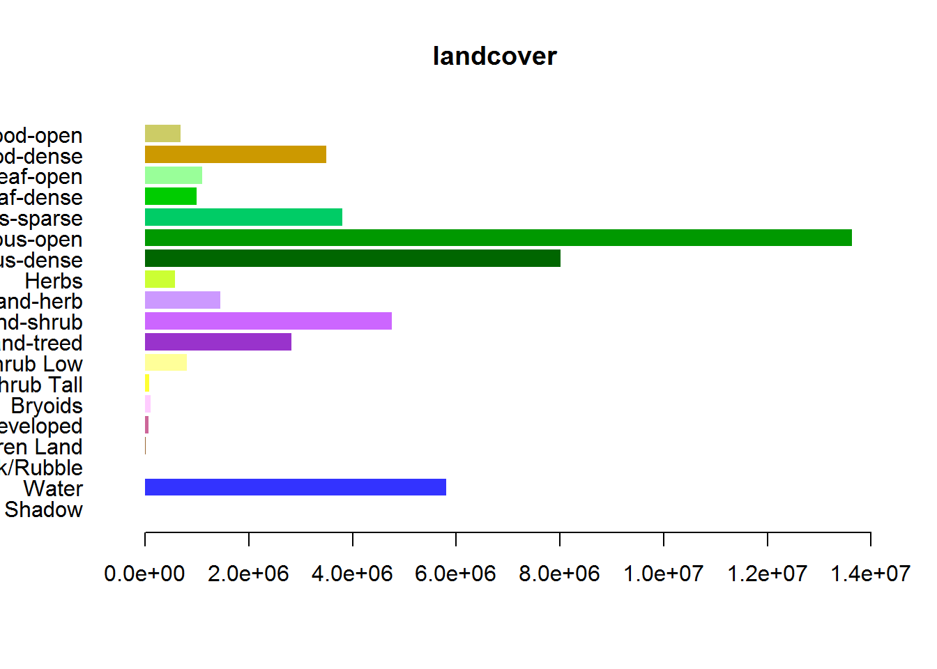
This is a useful figure.
2 Fire data
2.1 Loading the fire data
We will be adding fire data onto our existing raster of land cover data.
The fire data are in shape files, which we dumped into a directory called fire:
list.files("./_data/fire")## [1] "NFDB_poly_20170928_NT1_2016_HRL_clip.cpg"
## [2] "NFDB_poly_20170928_NT1_2016_HRL_clip.dbf"
## [3] "NFDB_poly_20170928_NT1_2016_HRL_clip.prj"
## [4] "NFDB_poly_20170928_NT1_2016_HRL_clip.sbn"
## [5] "NFDB_poly_20170928_NT1_2016_HRL_clip.sbx"
## [6] "NFDB_poly_20170928_NT1_2016_HRL_clip.shp"
## [7] "NFDB_poly_20170928_NT1_2016_HRL_clip.shp.xml"
## [8] "NFDB_poly_20170928_NT1_2016_HRL_clip.shx"To work with shape files, the best tool is the sf (simple features) package.
require(sf)sf is a standardized way to encode spatial vector data. All of the sf functions begin with “st_”. This makes it very easy to search through the available functions in the sf package. Just type “st_” and press tab to search.
Use st_read to load the polygon data:
fires <- st_read("./_data/fire")## Reading layer `NFDB_poly_20170928_NT1_2016_HRL_clip' from data source `C:\Users\Elie\Box Sync\caribou\NWT\rsf\primers\_data\Fire' using driver `ESRI Shapefile'
## Simple feature collection with 222 features and 26 fields
## geometry type: MULTIPOLYGON
## dimension: XYZ
## bbox: xmin: -1301880 ymin: 2381890 xmax: -1032998 ymax: 2677630
## epsg (SRID): NA
## proj4string: +proj=aea +lat_1=50 +lat_2=70 +lat_0=40 +lon_0=-96 +x_0=0 +y_0=0 +datum=NAD83 +units=m +no_defsThe read function retreives the simple features from a file or database. Note that st_read(“./data/fire”) only works because there’s only 1 shape file in directory “fire”. If there were more than one shape file then you would also have to specify the name of the file within the directory like this:
st_read(“./data/fire/NFDB_poly_20170928_NT1_2016_HRL_clip.shp”)
Again, these commands can be used to get a general idea of the data:
nrow(fires)## [1] 222names(fires)## [1] "SRC_AGENCY" "FIRE_ID" "FIRENAME" "YEAR" "MONTH"
## [6] "DAY" "REP_DATE" "DATE_TYPE" "DECADE" "SIZE_HA"
## [11] "CAUSE" "SOURCE" "METHOD" "MORE_INFO" "CFS_REF_ID"
## [16] "CFS_HA" "CFS_NOTE" "CFS_NOTE2" "ACQ_DATE" "AG_SRCFILE"
## [21] "POLY_DATE" "OUTDATE" "LAT" "LONG" "Shape_Leng"
## [26] "Shape_Area" "geometry"str(fires)## Classes 'sf' and 'data.frame': 222 obs. of 27 variables:
## $ SRC_AGENCY: Factor w/ 2 levels "AB","NWT": 1 2 2 2 2 2 2 2 2 2 ...
## $ FIRE_ID : Factor w/ 222 levels "1967HY-014","1968FS-018",..: 222 201 198 205 208 209 204 197 203 207 ...
## $ FIRENAME : Factor w/ 12 levels "2012FS009","2012FS021",..: NA NA NA NA NA NA NA NA NA NA ...
## $ YEAR : num 2008 2015 2015 2015 2015 ...
## $ MONTH : num 6 5 5 6 6 6 6 5 6 6 ...
## $ DAY : num 28 1 26 24 26 27 24 24 24 26 ...
## $ REP_DATE : Date, format: "2008-06-28" "2015-05-01" ...
## $ DATE_TYPE : Factor w/ 2 levels "Start date","Startdate": 1 NA NA NA NA NA NA NA NA NA ...
## $ DECADE : Factor w/ 6 levels "1960-1969","1970-1979",..: 5 6 6 6 6 6 6 6 6 6 ...
## $ SIZE_HA : num 170 1314 1012 6817 1884 ...
## $ CAUSE : Factor w/ 4 levels "H","L","n/a",..: 2 2 2 2 2 2 2 2 2 2 ...
## $ SOURCE : Factor w/ 6 levels "corrected airborne GPS",..: 1 3 2 3 3 3 3 3 3 3 ...
## $ METHOD : Factor w/ 0 levels: NA NA NA NA NA NA NA NA NA NA ...
## $ MORE_INFO : Factor w/ 0 levels: NA NA NA NA NA NA NA NA NA NA ...
## $ CFS_REF_ID: Factor w/ 222 levels "AB-2008-HWF136",..: 1 202 199 206 209 210 205 198 204 208 ...
## $ CFS_HA : num 550 1314 1012 6817 1884 ...
## $ CFS_NOTE : Factor w/ 2 levels "date and cause extracted from NWT point data",..: 2 NA NA NA NA NA NA NA NA NA ...
## $ CFS_NOTE2 : Factor w/ 1 level "see src agy data for mapped burn into adjacent agy": 1 NA NA NA NA NA NA NA NA NA ...
## $ ACQ_DATE : Date, format: "2012-05-08" "2015-11-26" ...
## $ AG_SRCFILE: Factor w/ 5 levels "2010 Final","2011Final",..: 5 NA NA NA NA NA NA NA NA NA ...
## $ POLY_DATE : Date, format: "2008-08-15" NA ...
## $ OUTDATE : Date, format: NA "2015-08-01" ...
## $ LAT : num 0 0 0 0 0 0 0 0 0 0 ...
## $ LONG : num 0 0 0 0 0 0 0 0 0 0 ...
## $ Shape_Leng: num 14883 14164 17623 38902 32729 ...
## $ Shape_Area: num 3821502 4385988 10120315 27724563 18844975 ...
## $ geometry :sfc_MULTIPOLYGON of length 222; first list element: List of 2
## ..$ :List of 1
## .. ..$ : num [1:5, 1:3] -1114541 -1114551 -1114647 -1114636 -1114541 ...
## ..$ :List of 1
## .. ..$ : num [1:108, 1:3] -1116761 -1116685 -1116643 -1116408 -1116310 ...
## ..- attr(*, "class")= chr "XYZ" "MULTIPOLYGON" "sfg"
## - attr(*, "sf_column")= chr "geometry"
## - attr(*, "agr")= Factor w/ 3 levels "constant","aggregate",..: NA NA NA NA NA NA NA NA NA NA ...
## ..- attr(*, "names")= chr "SRC_AGENCY" "FIRE_ID" "FIRENAME" "YEAR" ...Head shows you the first few rows of data, nrow tells you the number of rows and names shows you the name of each column.
2.2 Plotting the fire data (a bunch of ways)
Next, plot the data:
plot(fires)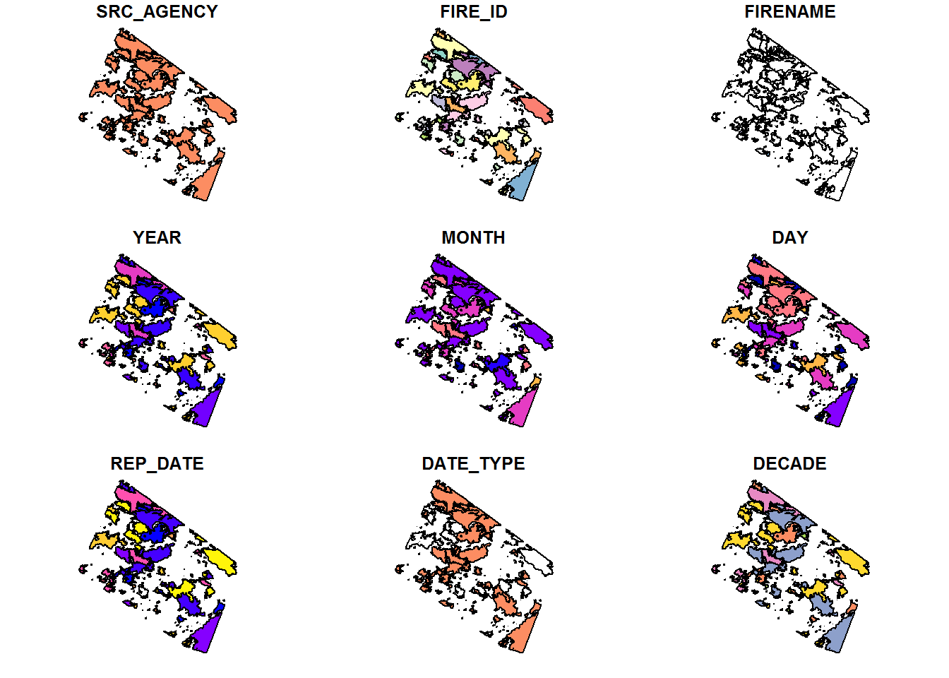
That gives you an awful lot of maps, but we just want one. To do that we need to specify which variables will be included, for example:
plot(st_geometry(fires), col = fires$YEAR)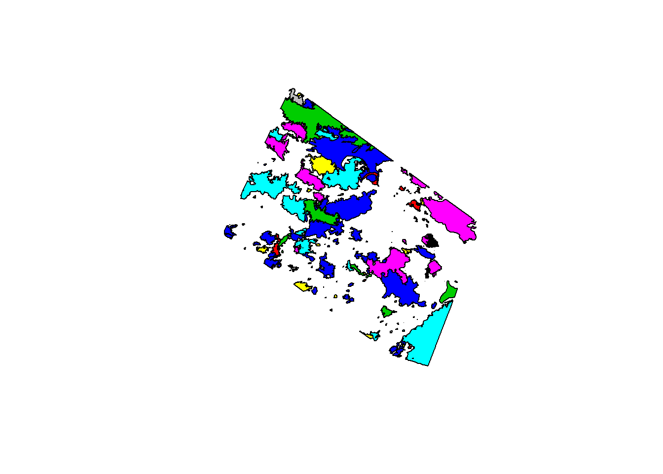
where st_geometry is used to get the geometry from an sf object.
2.2.1 Making a Color Palette
We want to know how recent the fires are, so the colors of each shape are based on the year. But these colors aren’t the most intuitive.
Here is one way to make a color palette that communicates the data a bit better:
range(fires$YEAR)## [1] 1967 2016palette(heat.colors(50))
plot(st_geometry(fires), col = fires$YEAR - 1966, border = "grey")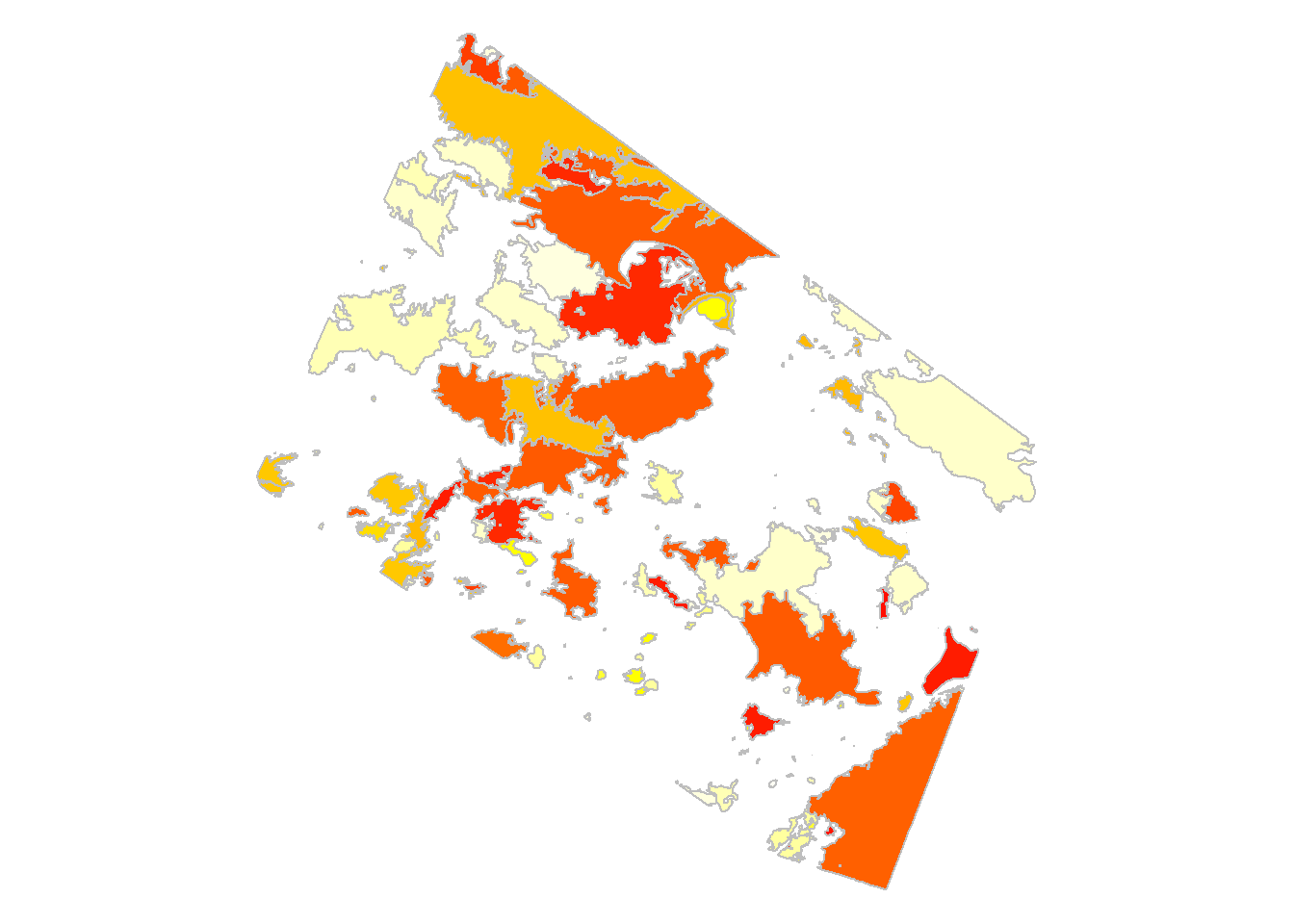
diff(range(fires$YEAR)) finds the difference between the first and last year in the dataset. Once we know that we use palette(heat.colors(50)) to split the palette into 50 distinct colors, one for each year. The heat.colors pallete ranges from red(1) to yellow(50). Because the oldest fire is from 1967, col = fires$YEAR - 1966 interprets it as red (1967 - 1966 = 1 = red).
One downside to the method above is that you can’t tell where fires overlap. Here is a way to see which areas have been burnt more than once:
require(scales)
plot(st_geometry(fires), col = alpha("red", 0.3), border = NA)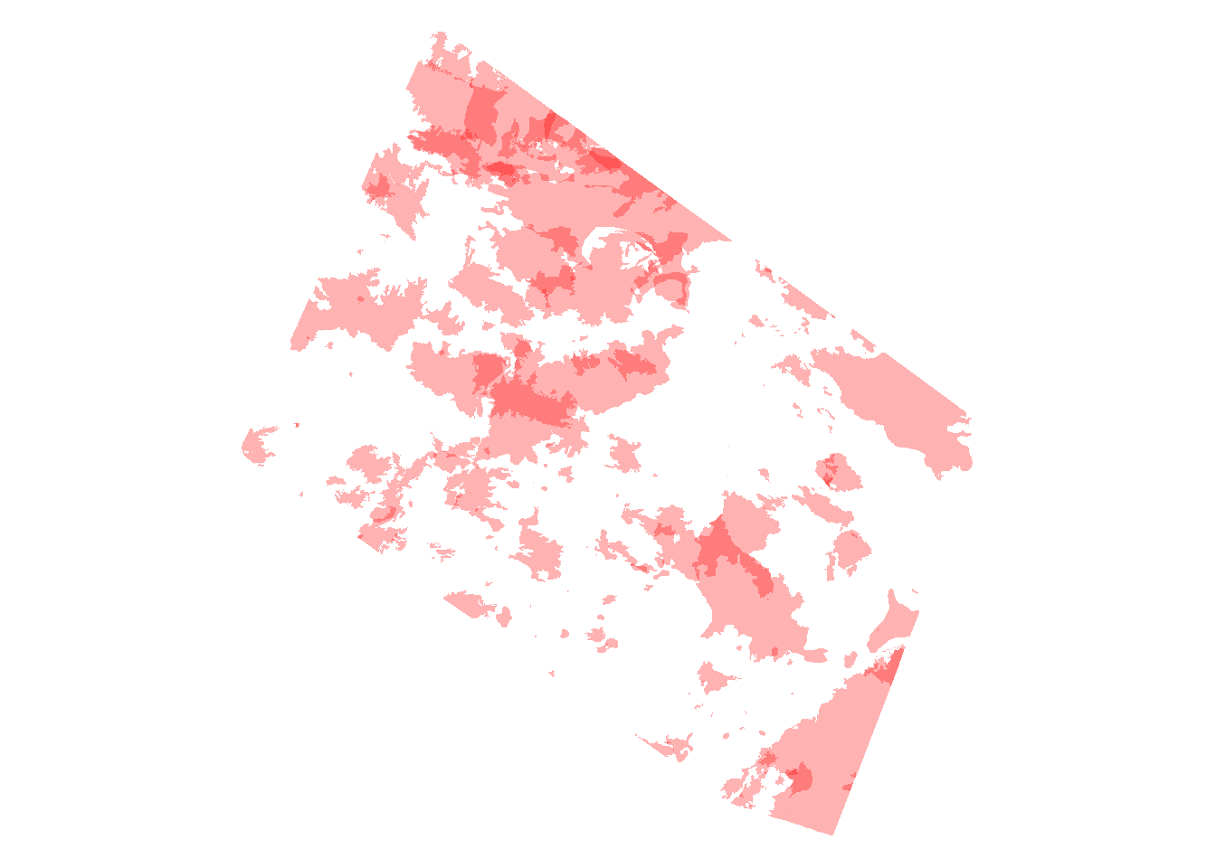
alpha adjusts the transparency of a color, where 1 = completely opaque and 0 = completely transparent. Where shapes overlap the color becomes more saturated. Here you can see that the areas that have burnt multiple times are a more saturated red. (You might need the scales package to use alpha).
Another way to look at the data is to separate the “recent” fires from the older ones:
fires$RECENT <- fires$YEAR > 2006
palette("default")
plot(st_geometry(fires), col = fires$RECENT + 3)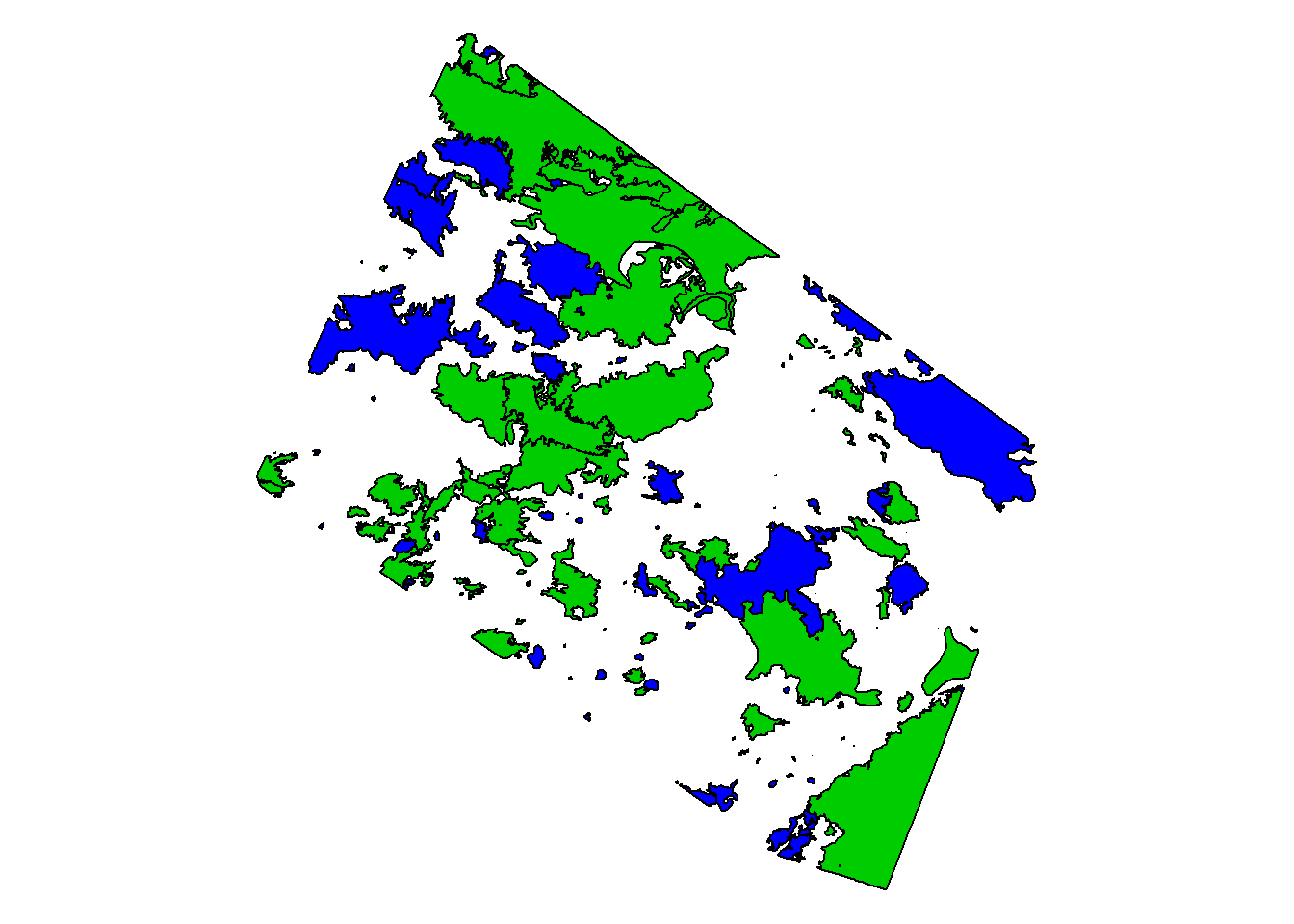
We defined “recent” as any year after 2006. fires$RECENT created a new attribute (aka column) within the shapefile. For each fire, if the year is greater than 2006 then the output is TRUE. If the year is 2006 or less then the output is FALSE.
2.2.2 Using ggplot
The ggplot2 package has some tools for visualizing simple feature data, e.g. (color coding by year):
require(ggplot2)
ggplot(fires) + geom_sf(aes(fill = YEAR))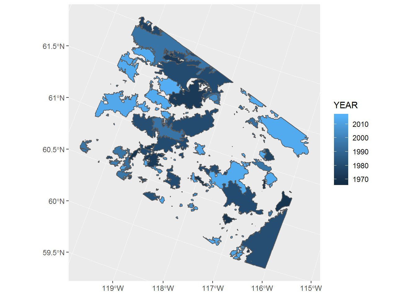
This is pretty compact! Here’s a version against decades (sorry for the Easter colors … those are ggplot defaults).
ggplot(fires) + geom_sf(aes(fill = DECADE))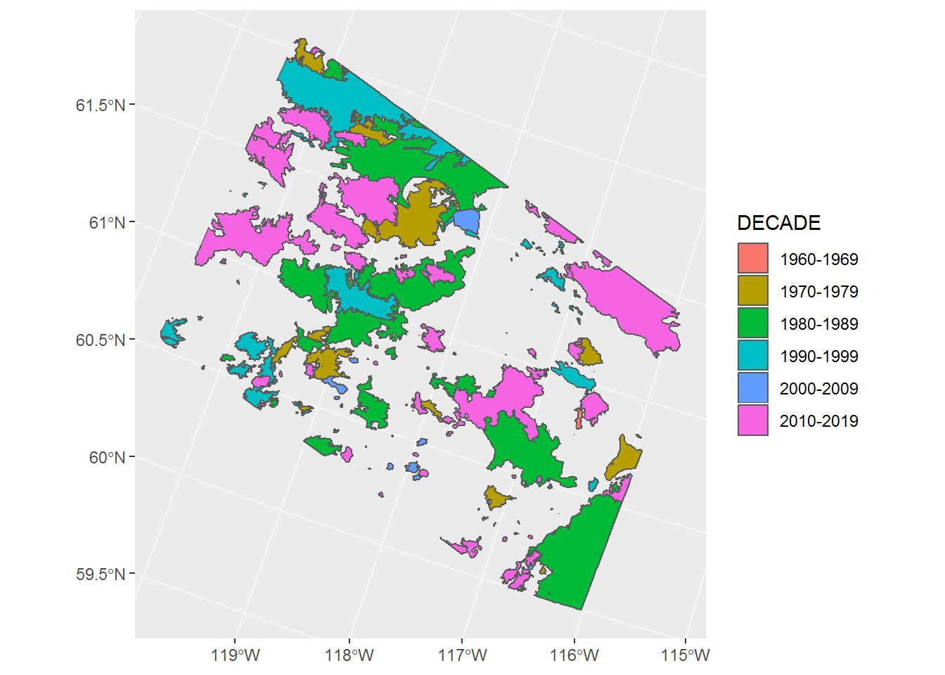
3 Combining fire and raster
3.1 Plotting both
The next thing we are going to do is convert our fire shapefile into a raster, and then plot that fire raster on top of our original land use raster. If we are going to draw these two files on top of each other, they need to have the same projection. Here is the fire projection:
st_crs(fires)## Coordinate Reference System:
## No EPSG code
## proj4string: "+proj=aea +lat_1=50 +lat_2=70 +lat_0=40 +lon_0=-96 +x_0=0 +y_0=0 +datum=NAD83 +units=m +no_defs"st_crs is a third way to find the projection (or coordinate reference system, same thing) this time using the sf package.
Is this the same as the raster?
projection(EOSD)## [1] "+proj=aea +lat_1=50 +lat_2=70 +lat_0=40 +lon_0=-112 +x_0=0 +y_0=0 +datum=NAD83 +units=m +no_defs +ellps=GRS80 +towgs84=0,0,0"No! They have different projections - both are Albers Equal Area, but the centering is different.
So, we transform the fire shapefile to give it the same projection as the EOSD raster:
fires.projected <- st_transform(fires, crs = projection(EOSD))And then the fire shapefile can be ploted on top of the land use raster. We’ll plot just the recent fires:
plot(EOSD) + plot(st_geometry(subset(fires.projected, RECENT)),
col = alpha("red", .5), add = TRUE)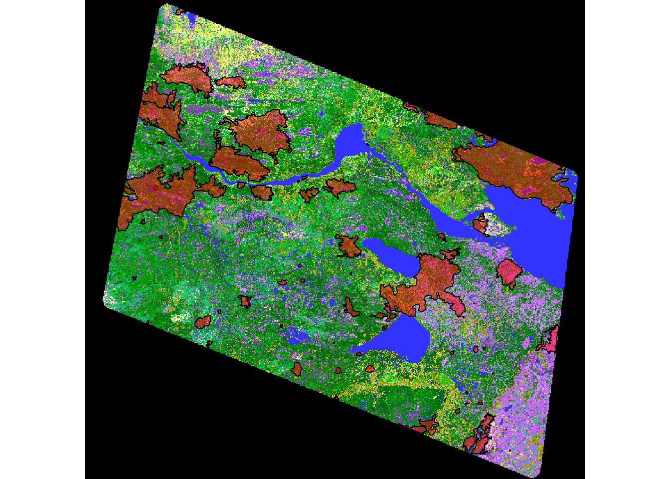
## integer(0)There you have it: land use and recent burn scars all in one map.
3.2 Converting a Shapefile to a Raster
Right now the fire data and the land use data are ploted together, but they are still two different layers with two different data types. If you want to actually merge the fire data into the original EOSD raster, first you need to convert the fire data from a shapefile into a raster.
We used to turn the shape files into rasters using rasterize. Here’s an example:
recentfire.sf <- st_zm(subset(fires.projected, RECENT))
recentfire.raster <- rasterize(recentfire.sf, EOSD.blank, field = c("FIRE_ID", "YEAR", "REP_DATE", "OUTDATE"))
plot(recentfire.raster)The st_zm function removes the Z and/or M dimensions from feature geometries. We are making a two-dimensional raster object so recentfires.sf should only have X and Y dimensions.
The second argument of rasterize is EOSD which contains the exact geometry (extent + projection + resolution) that we want for the new raster. Note also that we specified several fields that we thought might be worth keeping from the original polygon data.
This step takes a LOOONG time (e.g. > 5 min on a decent desktop - Might be worth doing in ArcGIS?). After it’s done, it is best to save the new raster using writeRaster. Depending on the file type you chose, your raster can take up a lot of memory. If you use .tif it will use much less space than .grd (which is the R raster data default format).
The first time we tried to do this, we got an error:
writeRaster(recentfire.raster, filename = "./_data/rasters/RecentFires.tif")Error in .checkLevels(levels(x)[[1]], value) :
the first column name of the raster attributes (factors) data.frame should be "ID"It was complaining that the first column of the attributes feature wasn’t called ID … it is called FIRE_ID. The best way to fix this is simply to add another column called ID that counts from 1 to the number of rows to the attributes of the new raster.
levels(recentfire.raster)[[1]] <- data.frame(ID = 1:nrow(levels(recentfire.raster)[[1]]), levels(recentfire.raster)[[1]])
writeRaster(recentfire.raster, filename = "./_data/rasters/RecentFires.tif")3.2.1 VERY IMPORTANT UPDATE!!!!
A brand new package called (wait for it) … fasterize rasterizes things faster. The following generates basically the same output, but licketysplit:
recentfire.sf <- st_zm(subset(fires.projected, RECENT))
require(fasterize)
EOSD.blank <- raster(EOSD)
recentfire.raster <- fasterize(recentfire.sf, EOSD.blank, field = "YEAR")
recentfire.raster <- ratify(recentfire.raster)
plot(recentfire.raster)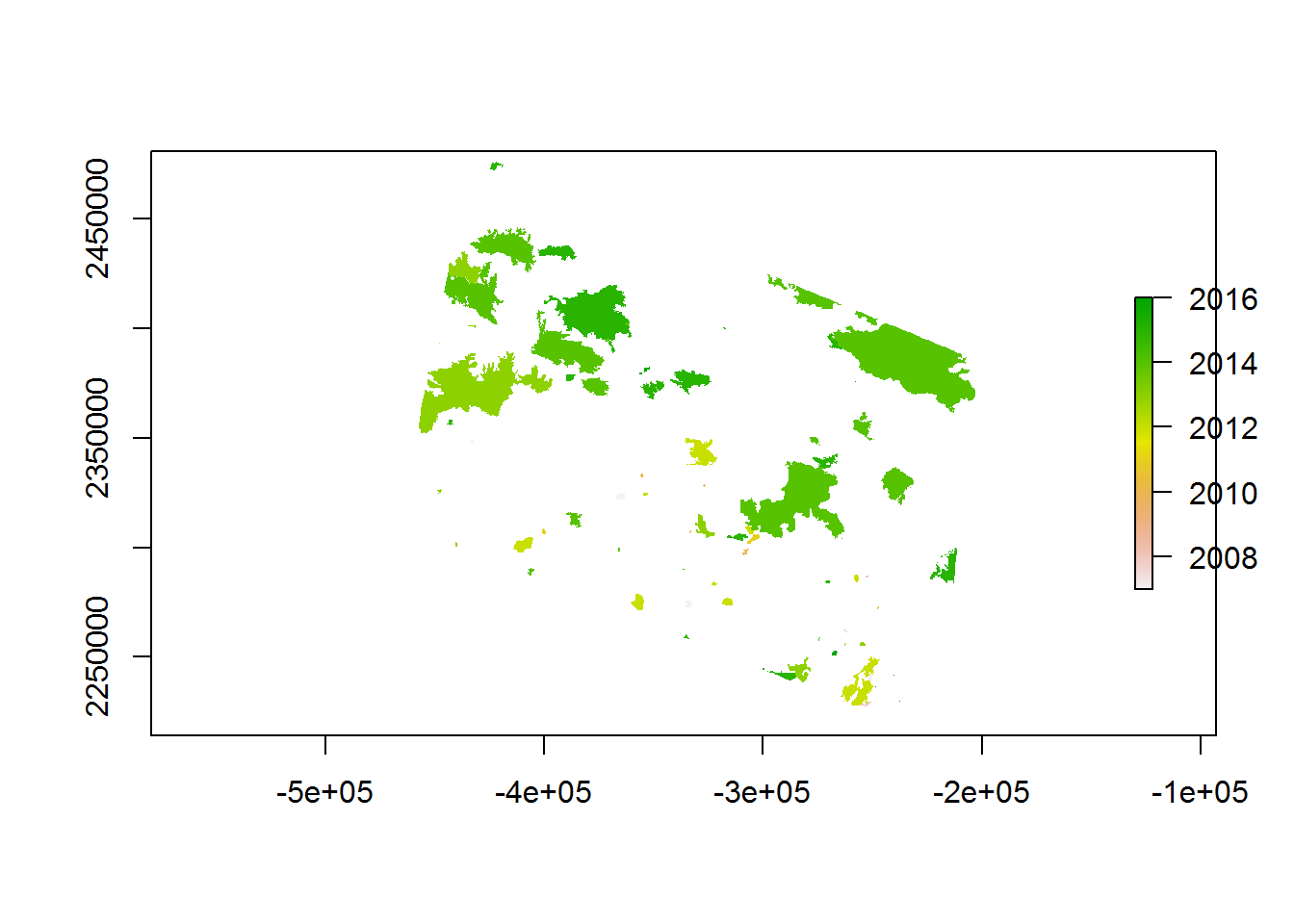
If multiple polygons overlap, fasterize (and that lousy, slow rasterize nonsense) will by default pick the LAST element in the list, but you can pick other functions, e.g. sum or mean. Just to make SURE that the latest burn is what you’re getting her, you should ORDER the recentfire.sf by YEAR. Here’s a slightly funkier plot:
recentfire.sf <- arrange(recentfire.sf, YEAR)
recentfire.raster <- fasterize(recentfire.sf, EOSD.blank, field = "YEAR")
require(rasterVis)
levelplot(recentfire.raster)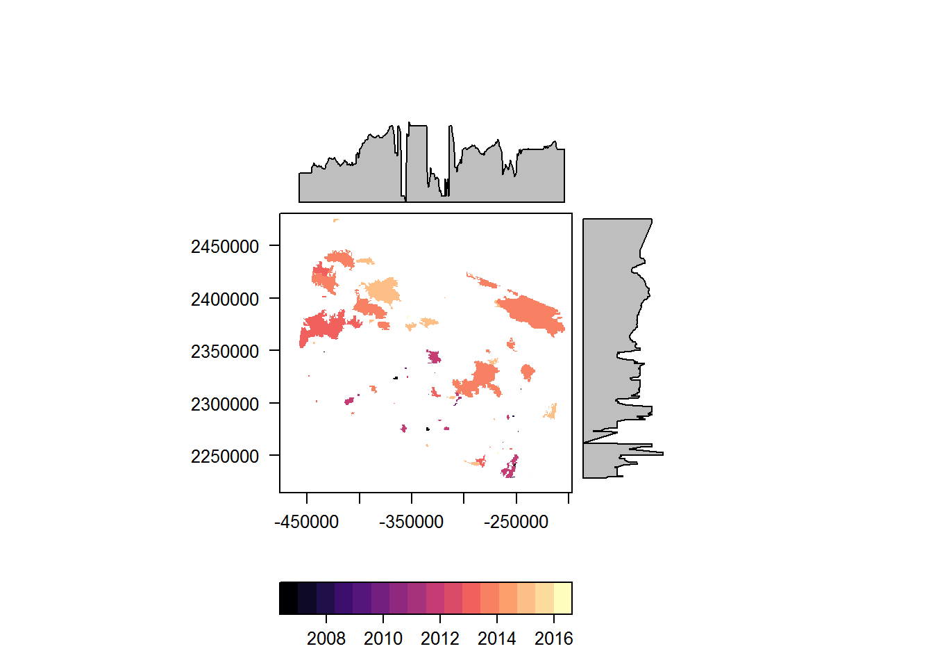
3.3 Adding a “fire” layer to the EOSD raster
Load the recent fires raster:
EOSD <- raster("./_data/rasters/EOSD_updated")
recentfire.raster <- raster("./_data/rasters/RecentFires.tif")
plot(recentfire.raster)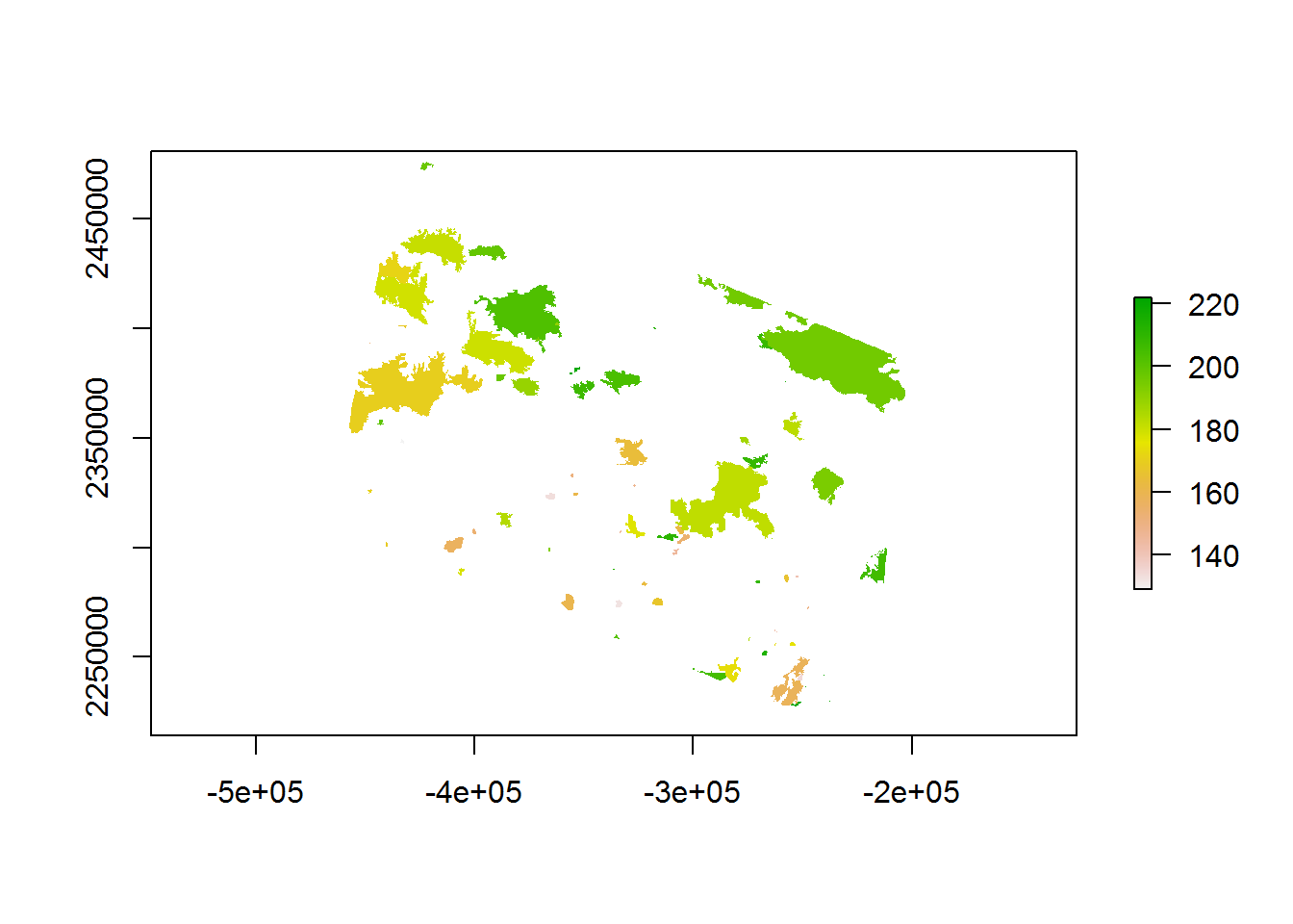
Our goal is to add a layer to the EOSD raster that corresponds to a recent burn. We have to choose a value to give to recent fire burns (lets make is 250 - which is not yet taken in the EOSD raster) and then, very simply, is to replace all non-NA fire locations in the EOSD raster with the value 250, and to modify the levels and colortable accordingly. We’ll do this to cropped versions of the EOSD and fire raster, to make things quicker:
cropextent <- extent(-411594.5, -384535.5, 2396389, 2419998)
EOSD.crop <- crop(EOSD, cropextent)
recentfire.raster.crop <- crop(recentfire.raster, cropextent)Find all non-NA locations in recentfires, and attribute new value (250) to those locations:
EOSD.withfire.crop <- EOSD.crop
EOSD.withfire.crop[!is.na(recentfire.raster.crop)] <- 250This is quite fast.
Adjust the color table (remember the +1!) - make it bright red (yes, Dean, I know actual forests look black when they’re burned, but this map needs more red):
EOSD.withfire.crop@legend@colortable[251] <- "#FF5555"Add another level to the EOSD data (by hand):
newlevels <- levels(EOSD.withfire.crop)[[1]]
newlevels <- rbind(newlevels, data.frame(ID = 19, OBJECTID = 20, Value = 250,
Description = "Recent Burn",
Color = EOSD.withfire.crop@legend@colortable[251],
Count = NA))
levels(EOSD.withfire.crop)[[1]] <- newlevelsAnd plot this new raster:
plot(EOSD.withfire.crop)
legend("topright", fill = levels(EOSD.crop)[[1]]$Color,
legend = levels(EOSD.crop)[[1]]$Description, ncol = 2, cex = 0.55)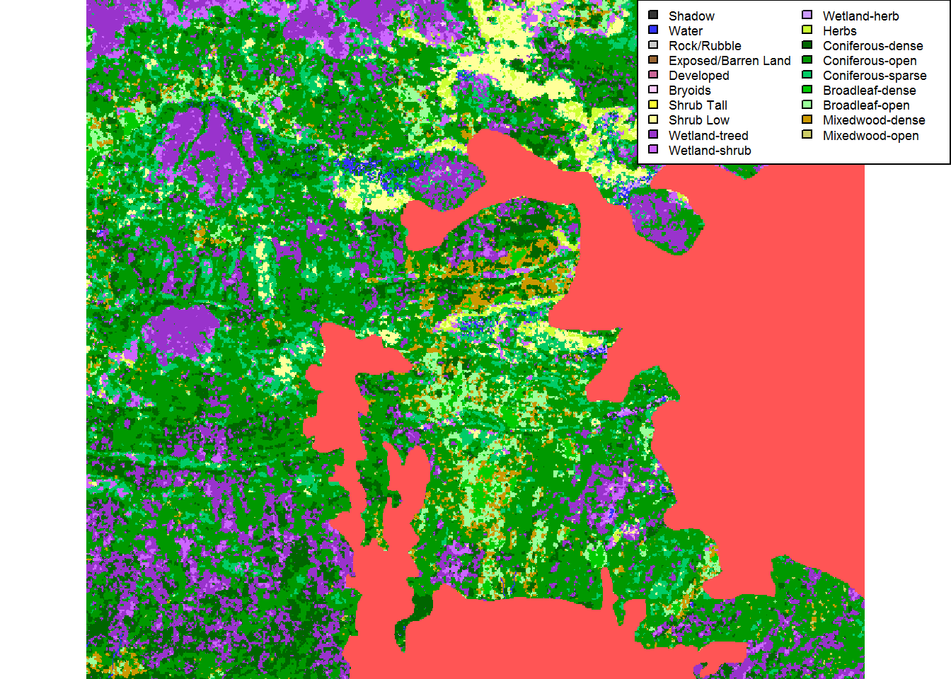
3.3.1 Updating the counts
We might want to update the counts (which are, anyways, not valid for the crop at all):
counts <- table(getValues(EOSD.withfire.crop))
counts.df <- data.frame(counts)
newlevels <- merge(levels(EOSD.withfire.crop)[[1]], counts.df, by.x = "Value", by.y = "Var1")This data frame contains the right counts, and only retains those landcover types that exist in this cropped raster, but needs to be transformed a bit to be made a valid levels for the raster.
require(plyr)
newlevels <- mutate(newlevels[c("ID", "OBJECTID", "Value", "Description", "Color", "Freq")],
Count = Freq, Freq = NULL)
levels(EOSD.withfire.crop)[[1]] <- newlevelsAnd a quick barplot of the levels:
par(mar = c(4,10,2,2), cex = 0.8, mgp = c(2,.5,0))
barplot(newlevels$Count, col = newlevels$Color,
horiz = TRUE, las = 1, bor = NA, names.arg = newlevels$Description, main = "landcover")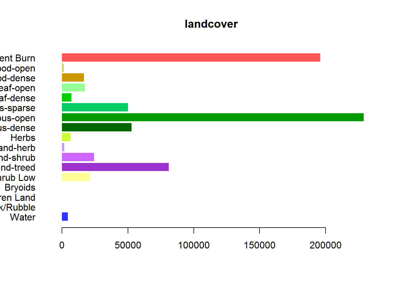
Clearly, this portion is dominated by the recent burn! Here are the exact proportions:
newlevels$Count## [1] 4419 11 5 24 21340 80965 24351 1748 6456 52932
## [11] 228898 50036 7257 17286 16774 1341 1960313.4 Performing all of the above on the complete raster
Below, we perform the entire loading and processing operations, and timing them (out of curiousity).
# load both rasters and update the levels
start.time <- Sys.time() # just to time this process
EOSD <- raster("./_data/EOSD/EOSD_NWT_HRL_clip.tif")
recentfire.raster <- raster("./_data/rasters/RecentFires.tif")
EOSD.legend <- read.delim("./_data/EOSD/EOSD_legend.txt", sep = "\t")
RGB.raw <- as.character(EOSD.legend$RGB.Code)
Colors <- sapply(strsplit(RGB.raw, ";"), function(x) rgb(x[1], x[2], x[3], maxColorValue = 255))
EOSD.legend$Color <- Colors
LevelsMerged <- merge(levels(EOSD)[[1]], EOSD.legend[,c("Value","Description","Color")], by = "Value", all.x = TRUE)
LevelsMerged <- LevelsMerged[,c("ID","OBJECTID","Value","Description","Color","Count")]
levels(EOSD)[[1]] <- LevelsMerged
EOSD@legend@colortable[EOSD.legend$Value+1] <- EOSD.legend$Color
loading.and.prepping.time <- Sys.time() - start.time
# update with recent burns and plot
start.time <- Sys.time()
EOSD.withfire <- EOSD
EOSD.withfire[!is.na(recentfire.raster)] <- 250
EOSD.withfire@legend@colortable[251] <- "#FF5555"
levels(EOSD.withfire)[[1]] <- rbind(levels(EOSD.withfire)[[1]], data.frame(ID = 19, OBJECTID = 20, Value = 250,
Description = "Recent Burn",
Color = EOSD.withfire@legend@colortable[251],
Count = NA))
adding.burns.time <- Sys.time() - start.time require(plyr)
start.time <- Sys.time()
# this is the super slow step
counts <- table(getValues(EOSD.withfire))
counts.df <- data.frame(counts)
newlevels <- merge(levels(EOSD.withfire)[[1]], counts.df, by.x = "Value", by.y = "Var1")
newlevels <- mutate(newlevels[c("ID", "OBJECTID", "Value", "Description", "Color", "Freq")],
Count = Freq, Freq = NULL)
levels(EOSD.withfire)[[1]] <- newlevels
counting.landcover.types.time <- Sys.time() - start.time plot(EOSD.withfire)
legend("topright", fill = levels(EOSD.withfire)[[1]]$Color,
legend = levels(EOSD.withfire)[[1]]$Description, ncol = 2, cex = 0.55)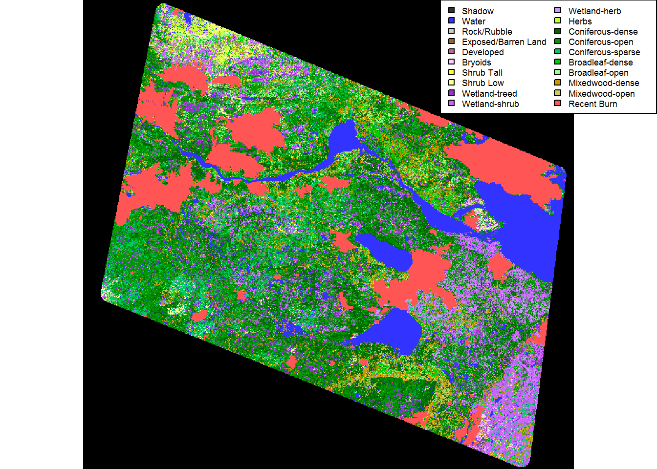
Here’s a barplot - a bit different than the others because I arranged by the count:
par(mar = c(4,10,2,2), cex = 0.8, mgp = c(2,.5,0))
with(arrange(levels(EOSD.withfire)[[1]], Count),
barplot(Count, col = Color, names = Description,
horiz = TRUE, las = 1, bor = NA, main = "landcover"))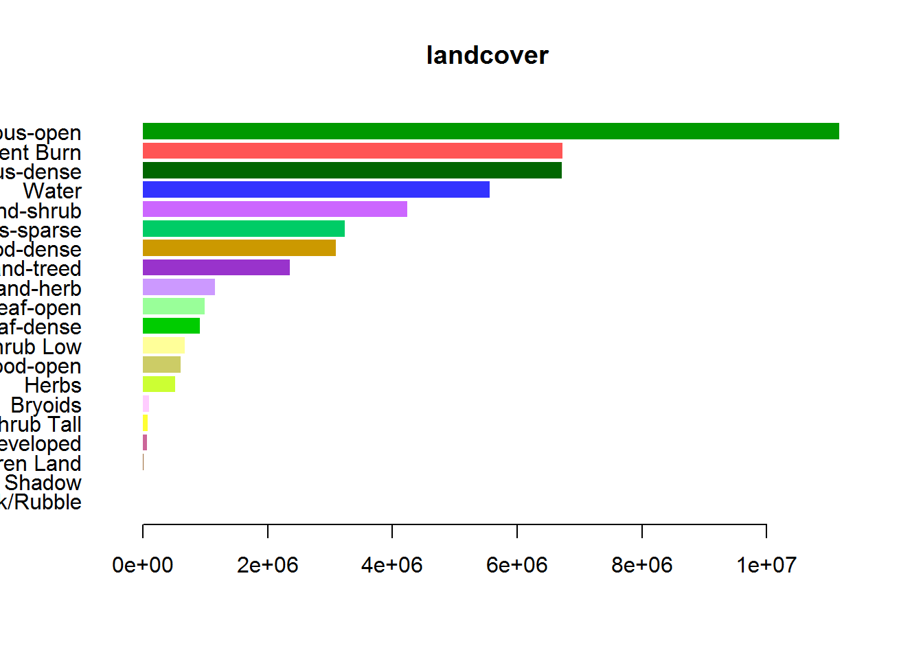
For reference, here are the computation times for htese steps (on an OK personal laptop):
data.frame(loading.and.prepping.time, adding.burns.time, counting.landcover.types.time)## loading.and.prepping.time adding.burns.time
## 1 0.03119993 secs 8.152 secs
## counting.landcover.types.time
## 1 1.00032 minsGiven the time it took to perform all these tasks, always best to SAVE YOUR RASTER!
writeRaster(EOSD.withfire, file = "./_data/rasters/EOSD_withfire.tif", options = c('TFW = YES'))4 Complete code
Click below to show complete code from this document.
knitr::opts_chunk$set(echo = TRUE, cache = TRUE, warning = FALSE)
pcks <- c("raster", "sf", "ggplot2", "plyr", "scales")
sapply(pcks, require, character = TRUE)
require(raster)
list.files("./_data/EOSD")
EOSD <- raster("./_data/EOSD/EOSD_NWT_HRL_clip.tif")
plot(EOSD)
EOSD
str(EOSD)
EOSD@crs
projection(EOSD)
EOSD@extent
bbox(EOSD)
EOSD@data@attributes[[1]]
levels(EOSD)[[1]]
(EOSD.legend <- read.delim("./_data/EOSD/EOSD_legend.txt", sep = "\t"))
RGB.raw <- as.character(EOSD.legend$RGB.Code)
Colors <- sapply(strsplit(RGB.raw, ";"), function(x) rgb(x[1], x[2], x[3], maxColorValue = 255))
EOSD.legend$Color <- Colors
str(levels(EOSD)[[1]])
str(EOSD.legend)
(LevelsMerged <- merge(levels(EOSD)[[1]], EOSD.legend[,c("Value","Description","Color")], by = "Value", all.x = TRUE))
LevelsMerged <- LevelsMerged[,c("ID","OBJECTID","Value","Description","Color","Count")]
levels(EOSD)[[1]] <- LevelsMerged
EOSD@legend@colortable
which.not.black <- which(EOSD@legend@colortable != "#000000")
cols.not.black <- EOSD@legend@colortable[which.not.black]
plot(1:length(cols.not.black), bg = cols.not.black, pch = 21, cex = 3, bty = "l", axes = FALSE, xlab = "", ylab = "")
text(1:length(which.not.black), 1:length(which.not.black), which.not.black, font = 2, cex = 0.8)
EOSD.crop <- crop(EOSD, extent(-411594.5, -384535.5, 2396389, 2419998))
plot(EOSD.crop)
EOSD.crop2 <- EOSD.crop
EOSD.crop2@legend@colortable[EOSD.legend$Value+1] <- EOSD.legend$Color
plot(EOSD.crop2)
EOSD@legend@colortable[EOSD.legend$Value+1] <- EOSD.legend$Color
## writeRaster(EOSD, file = "./_data/rasters/EOSD_updated.tif")
## writeRaster(EOSD, file = "./_data/rasters/EOSD_updated")
plot(EOSD, main = "EOSD in the Hay River Lowlands Clip")
legend("topright", fill = levels(EOSD)[[1]]$Color, legend = levels(EOSD)[[1]]$Description, ncol = 2, cex = 0.55)
counts <- table(getValues(EOSD))
counts
counts.df <- cbind(levels(EOSD)[[1]], Count2 = as.vector(counts))
par(mar = c(4,10,2,2), cex = 0.8)
with(counts.df,
barplot(Count, col = Color, names = Description,
horiz = TRUE, las = 1, bor = NA, main = "landcover"))
list.files("./_data/fire")
require(sf)
fires <- st_read("./_data/fire")
nrow(fires)
names(fires)
str(fires)
plot(fires)
plot(st_geometry(fires), col = fires$YEAR)
par(mar = c(0,0,0,0))
range(fires$YEAR)
palette(heat.colors(50))
plot(st_geometry(fires), col = fires$YEAR - 1966, border = "grey")
par(mar = c(0,0,0,0))
require(scales)
plot(st_geometry(fires), col = alpha("red", 0.3), border = NA)
par(mar = c(0,0,0,0))
fires$RECENT <- fires$YEAR > 2006
palette("default")
plot(st_geometry(fires), col = fires$RECENT + 3)
require(ggplot2)
ggplot(fires) + geom_sf(aes(fill = YEAR))
ggplot(fires) + geom_sf(aes(fill = DECADE))
st_crs(fires)
projection(EOSD)
fires.projected <- st_transform(fires, crs = projection(EOSD))
plot(EOSD) + plot(st_geometry(subset(fires.projected, RECENT)),
                  col = alpha("red", .5), add = TRUE)
## recentfire.sf <- st_zm(subset(fires.projected, RECENT))
## recentfire.raster <- rasterize(recentfire.sf, EOSD.blank, field = c("FIRE_ID", "YEAR", "REP_DATE", "OUTDATE"))
## plot(recentfire.raster)
## writeRaster(recentfire.raster, filename = "./_data/rasters/RecentFires.tif")
## levels(recentfire.raster)[[1]] <- data.frame(ID = 1:nrow(levels(recentfire.raster)[[1]]), levels(recentfire.raster)[[1]])
## writeRaster(recentfire.raster, filename = "./_data/rasters/RecentFires.tif")
recentfire.sf <- st_zm(subset(fires.projected, RECENT))
require(fasterize)
EOSD.blank <- raster(EOSD)
recentfire.raster <- fasterize(recentfire.sf, EOSD.blank, field = "YEAR")
recentfire.raster <- ratify(recentfire.raster)
plot(recentfire.raster)
recentfire.sf <- arrange(recentfire.sf, YEAR)
recentfire.raster <- fasterize(recentfire.sf, EOSD.blank, field = "YEAR")
require(rasterVis)
levelplot(recentfire.raster)
EOSD <- raster("./_data/rasters/EOSD_updated")
recentfire.raster <- raster("./_data/rasters/RecentFires.tif")
plot(recentfire.raster)
cropextent <- extent(-411594.5, -384535.5, 2396389, 2419998)
EOSD.crop <- crop(EOSD, cropextent)
recentfire.raster.crop <- crop(recentfire.raster, cropextent)
EOSD.withfire.crop <- EOSD.crop
EOSD.withfire.crop[!is.na(recentfire.raster.crop)] <- 250
EOSD.withfire.crop@legend@colortable[251] <- "#FF5555"
newlevels <- levels(EOSD.withfire.crop)[[1]]
newlevels <- rbind(newlevels, data.frame(ID = 19, OBJECTID = 20, Value = 250,
                                         Description = "Recent Burn",
                                         Color = EOSD.withfire.crop@legend@colortable[251],
                                         Count = NA))
levels(EOSD.withfire.crop)[[1]] <- newlevels
plot(EOSD.withfire.crop)
legend("topright", fill = levels(EOSD.crop)[[1]]$Color,
       legend = levels(EOSD.crop)[[1]]$Description, ncol = 2, cex = 0.55)
counts <- table(getValues(EOSD.withfire.crop))
counts.df <- data.frame(counts)
newlevels <- merge(levels(EOSD.withfire.crop)[[1]], counts.df, by.x = "Value", by.y = "Var1")
require(plyr)
newlevels <- mutate(newlevels[c("ID", "OBJECTID", "Value", "Description", "Color", "Freq")],
                    Count = Freq, Freq = NULL)

levels(EOSD.withfire.crop)[[1]] <- newlevels
par(mar = c(4,10,2,2), cex = 0.8, mgp = c(2,.5,0))
barplot(newlevels$Count, col = newlevels$Color,
        horiz = TRUE, las = 1, bor = NA,  names.arg = newlevels$Description, main = "landcover")
newlevels$Count
# load both rasters and update the levels
start.time <- Sys.time() # just to time this process

  EOSD <-  raster("./_data/EOSD/EOSD_NWT_HRL_clip.tif")
  recentfire.raster <- raster("./_data/rasters/RecentFires.tif")
  EOSD.legend <- read.delim("./_data/EOSD/EOSD_legend.txt", sep = "\t")

  RGB.raw <- as.character(EOSD.legend$RGB.Code)
  Colors <- sapply(strsplit(RGB.raw, ";"), function(x) rgb(x[1], x[2], x[3], maxColorValue = 255))
  EOSD.legend$Color <- Colors
  LevelsMerged <- merge(levels(EOSD)[[1]], EOSD.legend[,c("Value","Description","Color")], by = "Value", all.x = TRUE)
  LevelsMerged <- LevelsMerged[,c("ID","OBJECTID","Value","Description","Color","Count")]
  levels(EOSD)[[1]] <- LevelsMerged
  EOSD@legend@colortable[EOSD.legend$Value+1] <- EOSD.legend$Color

loading.and.prepping.time <- Sys.time() - start.time

# update with recent burns and plot
start.time <- Sys.time()

  EOSD.withfire <- EOSD
  EOSD.withfire[!is.na(recentfire.raster)] <- 250
  EOSD.withfire@legend@colortable[251] <- "#FF5555"
  levels(EOSD.withfire)[[1]] <- rbind(levels(EOSD.withfire)[[1]], data.frame(ID = 19, OBJECTID = 20, Value = 250,
                                           Description = "Recent Burn",
                                           Color = EOSD.withfire@legend@colortable[251],
                                           Count = NA))
adding.burns.time <- Sys.time() - start.time
require(plyr)
start.time <- Sys.time()
  # this is the super slow step
  counts <- table(getValues(EOSD.withfire))
  counts.df <- data.frame(counts)
  newlevels <- merge(levels(EOSD.withfire)[[1]], counts.df, by.x = "Value", by.y = "Var1")
  newlevels <- mutate(newlevels[c("ID", "OBJECTID", "Value", "Description", "Color", "Freq")],
                      Count = Freq, Freq = NULL)
  levels(EOSD.withfire)[[1]] <- newlevels
counting.landcover.types.time <- Sys.time() - start.time
  plot(EOSD.withfire)
  legend("topright", fill = levels(EOSD.withfire)[[1]]$Color,
         legend = levels(EOSD.withfire)[[1]]$Description, ncol = 2, cex = 0.55)
require(raster); require(plyr); EOSD.withfire <- raster("./_data/rasters/EOSD_withfire")
  par(mar = c(4,10,2,2), cex = 0.8, mgp = c(2,.5,0))
  with(arrange(levels(EOSD.withfire)[[1]], Count),
    barplot(Count, col = Color, names = Description,
            horiz = TRUE, las = 1, bor = NA, main = "landcover"))
data.frame(loading.and.prepping.time, adding.burns.time, counting.landcover.types.time)
## writeRaster(EOSD.withfire, file = "./_data/rasters/EOSD_withfire.tif", options = c('TFW = YES'))