Fitting and exploring RSF’s
Resource Selection Functions, Part III
Elie Gurarie
2019-11-29
The Goal: To fit resource selection models - from a straightforward logistic regression to more xomplex mixed effects models, up to and including a random slope model - to the Hay River woodland caribou data set.
A brief review of RSF’s
NOTE: An excellent introductory video lecture on RSF’s by John Fieberg (an expert in the field) is available at this link, and online materials are available here.
Most generally, a resource selection function is an approach to modeling spatial distribution of animal locations as a function of spatial covariates. In an RSF, we essentially model the (relative) probability of “use” of a particular location against the covariates that characterize the area. There are major asterisks associated with the use of the word “probability” here, since the actual probability of “use” is a difficult thing to define in the real world (e.g. the probability of being in a specific location at a specific time is - typically - very close to 0). With respect to the Used-Available design of our dataset, it depends entirely on the number of “available” points we collected for our sample.
The relative probability, however, is reasonably well-defined and useful. If an animal is 2 or 10 times more likely to be in a certain location, this gives us an important piece of information about the “quality” of the location.
The work-horse tool of RSF’s is - essentially - logistic regression, which is a general approach to modeling actual probabilities. The basic logistic regression formulation is: \[P(Y = 1) = {\exp(\beta_0 + \beta_1 X_1 + \beta_2 X_2 + ...) \over {1 + \exp(\beta_0 + \beta_1 X_1 + \beta_2 X_2 + ...)}}\]
where the \(X_i\)’s are the covariates we think are useful predictors, and the corresponding \(\beta\)’s are the coefficients that we are interested in. Positive values of \(\beta\) indicate higher probabilities of use, negative values indicate lower probabilities of use.
However, since we are not actually interested in probabilities (e.g. in the intercept of the logistic regression above) and our design is what might be called “used:available” design, it is perhaps more useful to model directly the following:
\[w_i(x, \beta) = \exp(\beta_1 x_1 + \beta_2 x_2 + \beta_3 x_3 + ...)\]
which has the advantage of being simpler (to look at), but does open up the question of what is \(w(x,\beta)\). The easiest way to think of this is as a “weighted distribution”, which gives weights to available locations in a way that generates a spatial distribution of used locations (Lele and Keim 2006). A more “modern” approach is to think of this function as a so-called “inhomogeneous Poisson process” (e.g. Muff et al. 2019), which is just a fancy way of saying that \(w\) models the probabilistic “intensity” of a point appearing in a given location.
All that stuff is relevant for interpreting the meaning of an RSF, but in any case the workhorse of actually estimating an RSF is simply logistic regression, and variants thereof (e.g., with random effects, splined bases, etc.) In the examples here, we will estimate the RSF for the Hay River population for which we prepped the data in the previous primer.
Hay River RSF - Three (or more) Ways
Load some useful packages and the formatted Hay River data (which we rename to the nice short hr).
pcks <- c("ggplot2", "plyr", "magrittr")
a <- sapply(pcks, require, character = TRUE)
load("_data/hayriver_RSF.rda")
hr <- hayriver.RSF
str(hr)
## 'data.frame': 9691 obs. of 11 variables:
## $ EOSD : num 211 82 81 212 211 81 82 83 212 83 ...
## $ nick_name : Factor w/ 13 levels "HR108","HR109",..: 1 1 1 1 1 1 1 1 1 1 ...
## $ timestamp : POSIXct, format: "2007-02-22 22:30:00" "2007-02-25 22:13:00" ...
## $ X : num -258895 -255315 -253800 -257247 -252508 ...
## $ Y : num 2255298 2265024 2267979 2264706 2262221 ...
## $ Road.Density: num 0 0.2148 0.0475 0.1892 0 ...
## $ DEM : num 301 302 308 304 296 ...
## $ Used : logi TRUE TRUE TRUE TRUE TRUE TRUE ...
## $ longitude : num -117 -117 -117 -117 -117 ...
## $ latitude : num 60.2 60.3 60.4 60.3 60.3 ...
## $ EOSD.class : Factor w/ 20 levels "Broadleaf-dense",..: 4 19 20 5 4 20 19 18 5 18 ...Logistic regression
We first fit a simple logistic regression model using EOSD.class, road density and a second order elevation polynomial to all of the data.
Note that when we perform the fitting, we need to compare our coefficients to a “reference class”, which - following Craig DeMars’ analysis - we always make Dense Conifer. To do this, we “relevel” the EOSD class column:
hr$EOSD.class = relevel(hr$EOSD.class, "Coniferous-dense")rsf1 <- glm(Used ~ scale(Road.Density) + scale(poly(DEM, 2)) + EOSD.class,
family = "binomial", data = hr)Note, we scale the continuous variables (i.e. subtract mean, divide by standard deviation) so that their contributions can be compared. We don’t need to do that to the categorical covariates, since those are internally encoded as “0’s” and “1”’s, so their “scale” is more or less comparable to that of the scaled covariates (whose means are 0 and standard deviations are 1).
The summary of this model outputs a whole bunch of coefficients and estimates
summary(rsf1)##
## Call:
## glm(formula = Used ~ scale(Road.Density) + scale(poly(DEM, 2)) +
## EOSD.class, family = "binomial", data = hr)
##
## Deviance Residuals:
## Min 1Q Median 3Q Max
## -2.5592 0.3183 0.3504 0.4063 6.1984
##
## Coefficients:
## Estimate Std. Error z value Pr(>|z|)
## (Intercept) 2.41545 0.09666 24.988 < 2e-16 ***
## scale(Road.Density) -0.05638 0.03941 -1.430 0.15260
## scale(poly(DEM, 2))1 -0.72166 0.09431 -7.652 1.98e-14 ***
## scale(poly(DEM, 2))2 -1.01803 0.15805 -6.441 1.19e-10 ***
## EOSD.classBroadleaf-dense -3.05014 0.71426 -4.270 1.95e-05 ***
## EOSD.classBroadleaf-open -2.85679 0.54401 -5.251 1.51e-07 ***
## EOSD.classBryoids -1.43004 1.15986 -1.233 0.21760
## EOSD.classConiferous-open 0.37431 0.12193 3.070 0.00214 **
## EOSD.classConiferous-sparse -0.22349 0.17625 -1.268 0.20479
## EOSD.classDeveloped -15.19489 229.58493 -0.066 0.94723
## EOSD.classMixedwood-dense -0.99701 0.19895 -5.011 5.41e-07 ***
## EOSD.classMixedwood-open -0.48874 0.35243 -1.387 0.16551
## EOSD.classRecent Burn -0.38414 0.15778 -2.435 0.01490 *
## EOSD.classShrub Low -0.71536 0.46083 -1.552 0.12058
## EOSD.classShrub Tall -15.19776 229.60853 -0.066 0.94723
## EOSD.classWater -2.67406 0.17471 -15.305 < 2e-16 ***
## EOSD.classWetland-herb 0.22063 0.18669 1.182 0.23728
## EOSD.classWetland-shrub 0.05486 0.14376 0.382 0.70274
## EOSD.classWetland-treed 0.53343 0.19365 2.755 0.00588 **
## ---
## Signif. codes: 0 '***' 0.001 '**' 0.01 '*' 0.05 '.' 0.1 ' ' 1
##
## (Dispersion parameter for binomial family taken to be 1)
##
## Null deviance: 5774.5 on 9690 degrees of freedom
## Residual deviance: 5055.9 on 9672 degrees of freedom
## AIC: 5093.9
##
## Number of Fisher Scoring iterations: 11Many of these are highly significant, including elevation (1st and 2nd order), and quite a few of the EOSD classes.
A useful package and function for neatly “corralling” the results of a model fit is broom:tidy
require(broom); tidy(rsf1, conf.int = TRUE)## # A tibble: 19 x 7
## term estimate std.error statistic p.value conf.low conf.high
## <chr> <dbl> <dbl> <dbl> <dbl> <dbl> <dbl>
## 1 (Intercept) 2.42 0.0967 25.0 8.23e-138 2.23 2.61
## 2 scale(Road.De~ -0.0564 0.0394 -1.43 1.53e- 1 -0.132 0.0230
## 3 scale(poly(DE~ -0.722 0.0943 -7.65 1.98e- 14 -0.907 -0.539
## 4 scale(poly(DE~ -1.02 0.158 -6.44 1.19e- 10 -1.33 -0.714
## 5 EOSD.classBro~ -3.05 0.714 -4.27 1.95e- 5 -4.62 -1.72
## 6 EOSD.classBro~ -2.86 0.544 -5.25 1.51e- 7 -3.98 -1.80
## 7 EOSD.classBry~ -1.43 1.16 -1.23 2.18e- 1 -3.50 1.58
## 8 EOSD.classCon~ 0.374 0.122 3.07 2.14e- 3 0.133 0.612
## 9 EOSD.classCon~ -0.223 0.176 -1.27 2.05e- 1 -0.564 0.129
## 10 EOSD.classDev~ -15.2 230. -0.0662 9.47e- 1 NA 20.8
## 11 EOSD.classMix~ -0.997 0.199 -5.01 5.41e- 7 -1.38 -0.599
## 12 EOSD.classMix~ -0.489 0.352 -1.39 1.66e- 1 -1.14 0.260
## 13 EOSD.classRec~ -0.384 0.158 -2.43 1.49e- 2 -0.691 -0.0716
## 14 EOSD.classShr~ -0.715 0.461 -1.55 1.21e- 1 -1.55 0.287
## 15 EOSD.classShr~ -15.2 230. -0.0662 9.47e- 1 NA 20.8
## 16 EOSD.classWat~ -2.67 0.175 -15.3 7.03e- 53 -3.02 -2.33
## 17 EOSD.classWet~ 0.221 0.187 1.18 2.37e- 1 -0.138 0.596
## 18 EOSD.classWet~ 0.0549 0.144 0.382 7.03e- 1 -0.227 0.338
## 19 EOSD.classWet~ 0.533 0.194 2.75 5.88e- 3 0.163 0.925which can be combined the GGally:ggcoef function to quickly visualize the results.
require(GGally)
ggcoef(tidy(rsf1, conf.int = TRUE) %>% subset(std.error < 200),
       sort = "ascending", exclude_intercept = TRUE) +
  ggtitle("Coefficients: Simple logistic model RSF")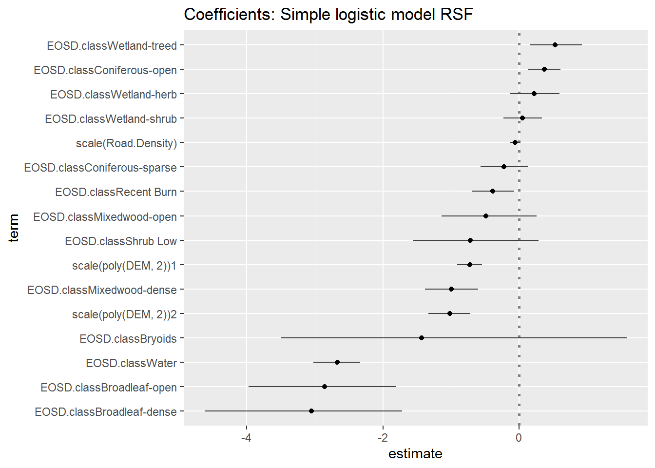
Note, I eliminated the poorly estimated variables (“tall shrub” and “developed”), which are anyways extremely rare in the data.
Recall that the ordered coefficient estimates are all presented relative to the reference land-cover class (Dense Conifer). Changing the reference class should have no effect on the ordering of the (factorial) effects. Below (using some extreme piping) I fit and plot the coefficients with no intercept - fitted by adding -1 to the formula:
glm(Used ~ scale(Road.Density) + scale(poly(DEM, 2)) + EOSD.class - 1, family = "binomial", data = hr) %>% tidy(conf.int = TRUE) %>% subset(std.error < 200) %>% ggcoef(sort = "ascending", exclude_intercept = TRUE) + ggtitle("Coefficients: Simple logistic model RSF - no intercept")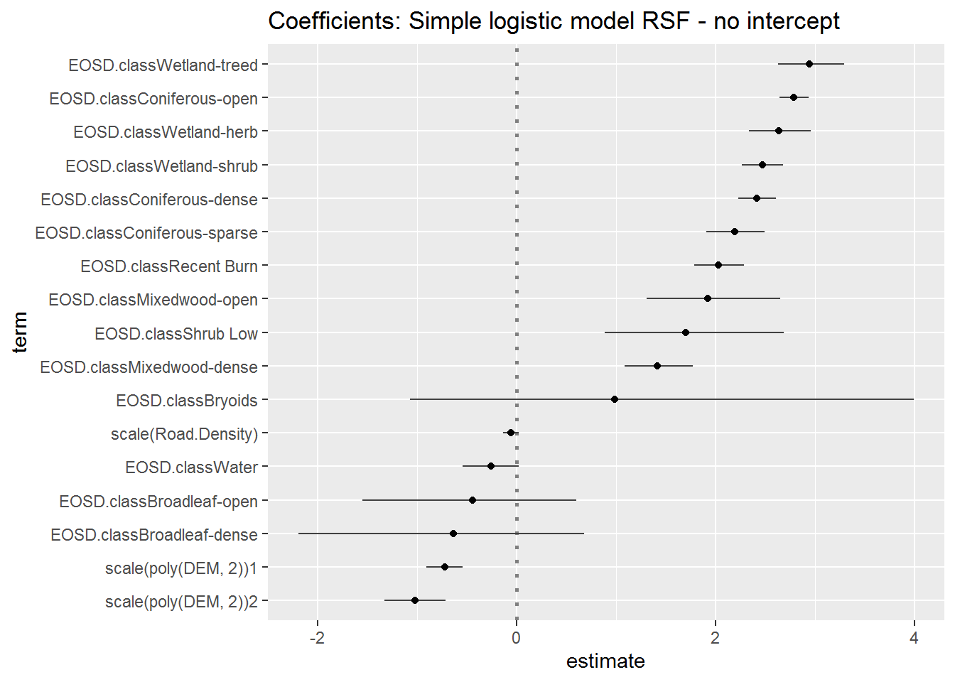
Again, the absolute value for the factorial coefficients are not actually important - since they really just reflect the number of Used vs. Available which we defined ourselvs (in this case there are 10x more Used - therefore the coefficients are mainly positive, whereas using the Dense Conifer class as a reference led to more negative coefficients). Note, however, that the continuous coefficients (elevation and road density) are stable - and their values are, in fact, telling - i.e. negative values really indicate “avoidance”.
For a bit more control, here’s a version below using straight ggplot, where I also rename the terms, plot in terms of ascending “preference”, color code by significance, and separate the continous from categorical covariates. Note, I use here (and moving forward) the no-intercept model:
rsf.glm <- glm(Used ~ scale(Road.Density) + scale(poly(DEM, 2)) + EOSD.class - 1,
            family = "binomial", data = hr)
rsf.coefs <- tidy(rsf.glm, conf.int = TRUE) %>%
subset(std.error < 200) %>%
mutate(type = ifelse(grepl("EOSD", term), "land-cover", "continuous"),
term = gsub("EOSD.class", "", term),
significance = cut(p.value, c(0,.01,.05,.1,1))) %>%
mutate(term = factor(term, levels = term[order(estimate)]))
ggplot(rsf.coefs, aes(estimate, term, xmin = conf.low, xmax = conf.high, col = significance)) +
geom_errorbarh() + geom_point() + geom_vline(xintercept = 0, lty = 3, lwd = 1) +
facet_wrap(.~type, scales = "free_y", ncol = 1) + scale_colour_hue(l = 40)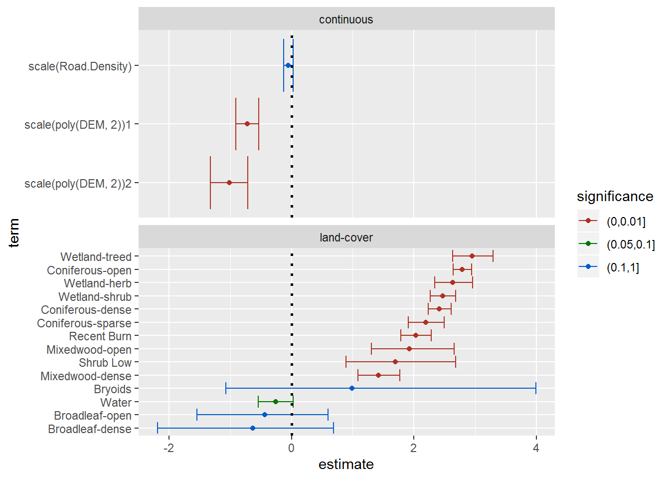
A few quick comments from these results:
The negative value for the second-order elevation term indicates that there is an “optimum” intermediate preferred elevation (the parabola is facing downward).
I color-coded by significance, but - again - for the categorical variables it is more instructive to look at the 95% error bars, and where they overlap. Thus, Water is very significantly avoided relative to most of the other land cover types (despite the individual p-value), and, similarly, despite their large confidence intervals - which reflect low abundance - (see: (https://terpconnect.umd.edu/~egurarie/research/NWT/Step07_RSF_PartII.html#land-cover_use)[Step07_RSF_PartII.html#land-cover_use]) - broadleaf categories are also largely avoided.
Mixed effects model: Random Intercept
Using the (fast and good-at-converging) glmmTMB package, we can add a random intercept (individual as a random effect). Note that first we have to add some ID identifications to the available locations.
require("glmmTMB")
hr[!hr$Used,]$nick_name <- sample(levels(hr$nick_name), sum(!hr$Used), replace = TRUE)
rsf.tmb <- glmmTMB(Used ~ EOSD.class + scale(Road.Density) + scale(poly(DEM, 2)) - 1 + (1|nick_name), family = "binomial", data = hr)
The summary of this fit is a bit more complex than for a simple glm:
summary(rsf.tmb)## Family: binomial ( logit )
## Formula:
## Used ~ EOSD.class + scale(Road.Density) + scale(poly(DEM, 2)) -
## 1 + (1 | nick_name)
## Data: hr
##
## AIC BIC logLik deviance df.resid
## 4273.6 4417.2 -2116.8 4233.6 9671
##
## Random effects:
##
## Conditional model:
## Groups Name Variance Std.Dev.
## nick_name (Intercept) 1.622 1.274
## Number of obs: 9691, groups: nick_name, 13
##
## Conditional model:
## Estimate Std. Error z value Pr(>|z|)
## EOSD.classConiferous-dense 1.80892 0.36892 4.903 9.42e-07 ***
## EOSD.classBroadleaf-dense -1.40154 0.97085 -1.444 0.14885
## EOSD.classBroadleaf-open -0.62636 0.67022 -0.935 0.35002
## EOSD.classBryoids 0.78692 1.24660 0.631 0.52787
## EOSD.classConiferous-open 2.03369 0.36270 5.607 2.06e-08 ***
## EOSD.classConiferous-sparse 1.39477 0.39092 3.568 0.00036 ***
## EOSD.classDeveloped -16.18395 2468.20214 -0.007 0.99477
## EOSD.classMixedwood-dense 0.83551 0.40595 2.058 0.03957 *
## EOSD.classMixedwood-open 1.28696 0.50896 2.529 0.01145 *
## EOSD.classRecent Burn 1.76782 0.38528 4.588 4.47e-06 ***
## EOSD.classShrub Low 1.42067 0.63136 2.250 0.02444 *
## EOSD.classShrub Tall -19.92192 8327.35413 -0.002 0.99809
## EOSD.classWater -0.76233 0.39184 -1.946 0.05171 .
## EOSD.classWetland-herb 1.79447 0.39266 4.570 4.88e-06 ***
## EOSD.classWetland-shrub 1.70433 0.37172 4.585 4.54e-06 ***
## EOSD.classWetland-treed 2.15030 0.39661 5.422 5.90e-08 ***
## scale(Road.Density) 0.18613 0.04508 4.129 3.65e-05 ***
## scale(poly(DEM, 2))1 -1.52119 0.12300 -12.367 < 2e-16 ***
## scale(poly(DEM, 2))2 -1.70942 0.19408 -8.808 < 2e-16 ***
## ---
## Signif. codes: 0 '***' 0.001 '**' 0.01 '*' 0.05 '.' 0.1 ' ' 1The coefficient estimates are obtained as follows (note tidy does not work for glmmTMB output):
coefs.tmb <- summary(rsf.tmb)$coef$cond %>% as.data.frameComparing fits visually. The code below mainly rearranges and combines results in preparation for the ggplot. Note that this time, I decided to order the covariates by their abundance in the landscape:
require(broom)
coefs.glm <- tidy(rsf.glm)
names(coefs.tmb) <- names(coefs.glm)[-1]
coefs.tmb$term <- row.names(coefs.tmb)

require(gtools)
# stack the two sets of coefficients into a "long" data frame
coefs.long <- smartbind(data.frame(model = "glm", coefs.glm),
                        data.frame(model = "glmmTMB", coefs.tmb))
coefs.long <- mutate(coefs.long, term = gsub("EOSD.class", "", term)) %>%
  mutate(term = gsub("scale(", "", term, fixed = TRUE)) %>%
  mutate(term = gsub(")", "", term, fixed = TRUE)) %>%
  mutate(term = ifelse(grepl(21, term), "DEM", ifelse(grepl(22, term), "DEM^2", term) )) %>%
  mutate(low = estimate - 2*std.error, high = estimate + 2*std.error,
         type = ifelse(grepl("DEM", term) | grepl("Road", term),
                                      "continuous", "landcover"))


EOSD.ordered <- names(table(subset(hr, !Used)$EOSD.class) %>% sort %>% {.; .[.>0]})
coefs.long$term <- factor(coefs.long$term, levels = c(EOSD.ordered, "DEM", "DEM^2", "Road.Density"))

ggplot(coefs.long %>% subset(std.error < 1e2),
       aes(estimate, term, col = p.value < 0.05)) +
             geom_errorbarh(aes(xmin = low, xmax = high)) +
       geom_vline(xintercept = 0, lty = 3, lwd = 1) +
       facet_grid(type~model, scales = "free_y") +
  geom_point()  + scale_colour_hue(l = 40)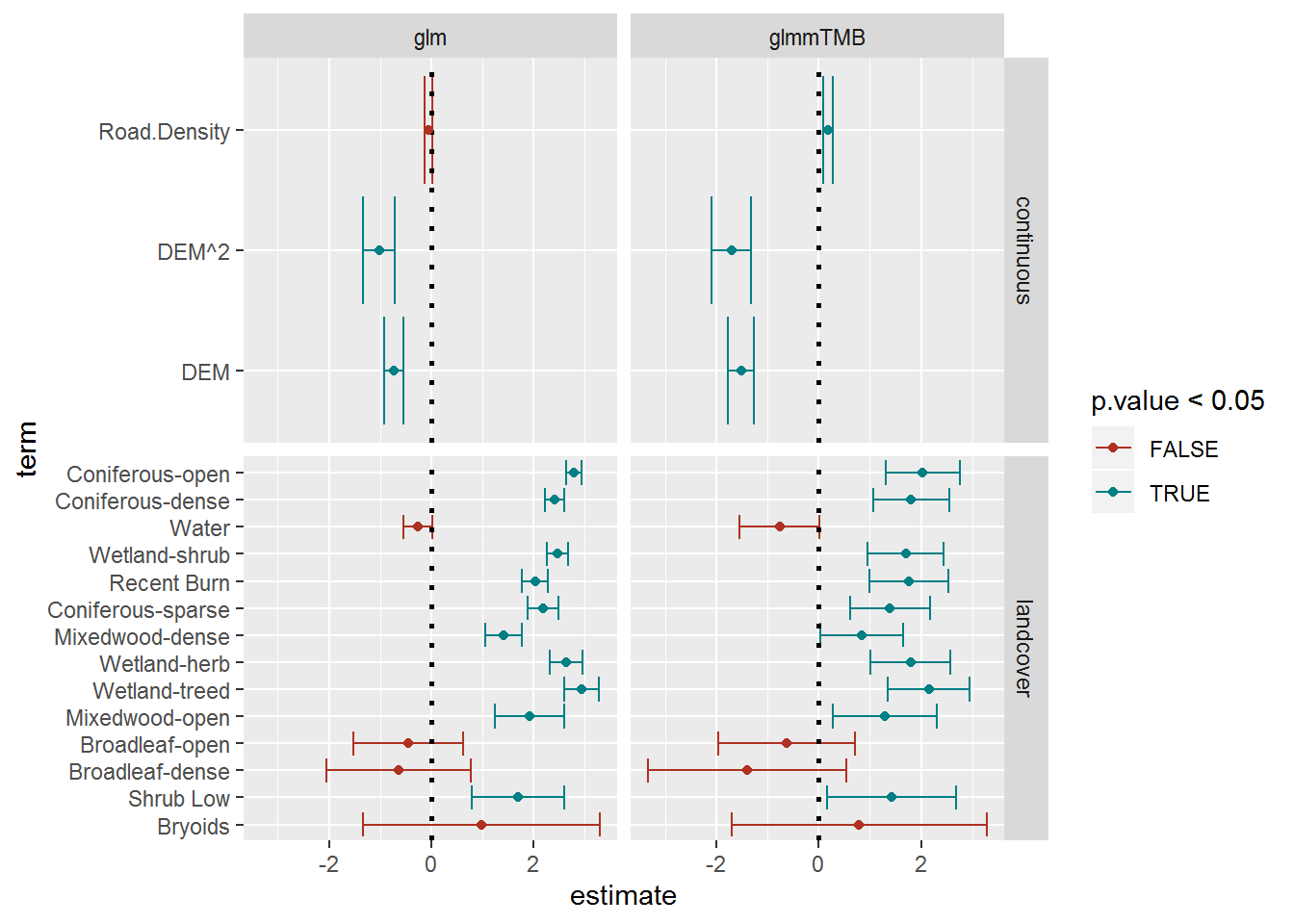
This comparison is highly instructive. The point estimates themselves are generally similar, but (as is typical of accounting for random effects) the mixed effects model coefficients are less precise (i.e. smaller error bars) than the “straight” glm. This is because the preferences of a single animal are observed over and over again and considered independent observations, whereas in fact they over-represent. The mixed effects model is more believable, and indicates that among the variaous land-class factors there is, in fact, less difference than we might first have been led to expect. On the other hand, the continous variable coefficients are apparently even more significant.
Note, incidentally, that the variability among individuals is quite high:
summary(rsf.tmb)$varcor # %>% names##
## Conditional model:
## Groups Name Std.Dev.
## nick_name (Intercept) 1.2737Mixed effects model: Random Slope
require("glmmTMB")
rsf.tmb.rs <- glmmTMB(Used ~ EOSD.class + scale(Road.Density) + scale(poly(DEM, 2)) - 1 +
                              (scale(Road.Density) + scale(DEM))|nick_name),
                            family = "binomial", data = hr)
A few things to note: (a) I only used first-order DEM, mainly because the second order version didn’t converge by trial and error, but also the first-order DEM random slope model had a much lower AIC than the second-order DEM random slope model; (b) the entire random effects portion here needs to be separated by parentheses, otherwise the function will pull in ALL Of the fixed effects into the random portion, and (c) fitting this model takes quite a bit longer than the other models, hence I’ve saved it and load it below.
load("_data/HR_rsf_tmb_randomslope.rda")Once again, we compare the coefficients three ways as above:
coefs.tmb.rs <- summary(rsf.tmb.rs)$coef$cond %>% as.data.frame
names(coefs.tmb.rs) <- names(coefs.glm)[-1]
coefs.tmb.rs$term <- row.names(coefs.tmb.rs)

coefs.long <- smartbind(data.frame(model = "glm", coefs.glm),
                        data.frame(model = "glmmTMB", coefs.tmb),
                        data.frame(model = "glmmTMB_randomslope", coefs.tmb.rs))

coefs.long <- mutate(coefs.long, term = gsub("EOSD.class", "", term)) %>%
  mutate(term = gsub("scale(", "", term, fixed = TRUE)) %>%
  mutate(term = gsub(")", "", term, fixed = TRUE)) %>%
  mutate(term = ifelse(grepl(21, term), "DEM", ifelse(grepl(22, term), "DEM^2", term) )) %>%
  mutate(low = estimate - 2*std.error, high = estimate + 2*std.error,
         type = ifelse(grepl("DEM", term) | grepl("Road", term),
                                      "continuous", "landcover"))

EOSD.ordered <- names(table(subset(hr, !Used)$EOSD.class) %>% sort %>% {.; .[.>0]})
coefs.long$term <- factor(coefs.long$term, levels = c(EOSD.ordered, "DEM", "DEM^2", "Road.Density"))

ggplot(coefs.long %>% subset(std.error < 1e2),
       aes(estimate, term, col = p.value < 0.05)) +
             geom_errorbarh(aes(xmin = low, xmax = high)) +
       geom_vline(xintercept = 0, lty = 3, lwd = 1) +
       facet_grid(type~model, scales = "free_y") +
  geom_point()  + scale_colour_hue(l = 40)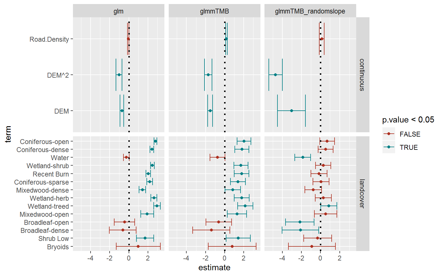
Overall, similar patterns (though a lower magnitude for unclear - to me - reasons), and, as expected, somewhat wider confidence intervals. The biggest change occurred in the continuous parameters - with the elevation coefficient much more negative.
require(reshape2)
estimates <- coefs.long[,c("model", "term", "type",  "estimate")] %>% dcast(term + type ~ model)
ggpairs(subset(estimates,
               pmin(glm, glmmTMB, glmmTMB_randomslope) > -10 &
                  type != "continuous")[,-(1:2)])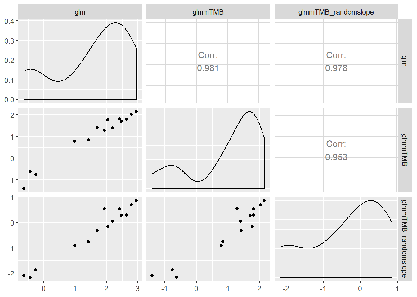
The magnitudes of the random effects are always worth checking out, since they show at a glance how individually variable animals are with respect to their RSF response.
summary(rsf.tmb.rs)$varcor##
## Conditional model:
## Groups Name Std.Dev. Corr
## nick_name (Intercept) 1.32169
## scale(Road.Density) 0.42797 0.050
## scale(DEM) 2.51242 0.184 -0.621These numbers are quite large relative to the point estimates.
Assessing and selecting models
The most common way to compare models is with an information criterion, especially AIC. We might ask - straightforwardly - whether it is even worth including road density, which is non-significant in most models we fit.
rsf.tmb.rs.RoadEOSD <- glmmTMB(Used ~ EOSD.class + Road.Density + poly(DEM, 2) + (DEM|nick_name),
                            family = "binomial", data = hr)
rsf.tmb.rs.noRoad <- glmmTMB(Used ~ EOSD.class + poly(DEM, 2) + (DEM|nick_name),
                            family = "binomial", data = hr)
rsf.tmb.rs.noEOSD <- glmmTMB(Used ~ Road.Density + poly(DEM, 2) + (DEM|nick_name),
                            family = "binomial", data = hr)

AIC(rsf.tmb.rs.RoadEOSD, rsf.tmb.rs.noRoad, rsf.tmb.rs.noEOSD)
## df AIC
## rsf.tmb.rs.RoadEOSD 22 3561.151
## rsf.tmb.rs.noRoad 21 3572.236
## rsf.tmb.rs.noEOSD 7 3759.514The lower AIC of the model with roads and with EOSD suggests that it is worth retaining both of those variables.
However, AIC is not a good tool for comparing mixed models with different random effect structure, since there is debate about how many degrees of freedom you assign to a random effect. More precisely, you have to know exactly what aspect of the model you want to be “best” - and that gets confusing. Here’s a discussion.
There are ways to assess the “goodness-of-fit” using a (generalized linear mixed model) equivalant of the familiar R^2 term. These are conveniently available in the (new to me and very useful) performance package. For GLMM, one can compute a marginal R^2 and a conditional R^2 - which basically assess how much of the variation is explained by the fixed effects, and by both the fixed and random effects, respectively. The key reference for this is Nakagawa and Schielzeth (2013). Here’s the computation:
require(performance)
# random intercept model
r2(rsf.tmb)
## # R2 for mixed models
##
## Conditional R2: 0.630
## Marginal R2: 0.630# random slope model
r2(rsf.tmb.rs)## # R2 for mixed models
##
## Conditional R2: 0.906
## Marginal R2: 0.901By this metric, the random slope model is terrifically better.
Incidentally, the performance package also has other useful tools for assessing the quality of a complex model. For example, a test of collinearity of the covariates:
check_collinearity(rsf.tmb.rs)## # Check for Multicollinearity
##
## Low Correlation
##
## Parameter VIF Increased SE
## EOSD.class 1.15 1.07
## scale(Road.Density) 1.48 1.22
## scale(poly(DEM, 2)) 1.63 1.28This is a reassuring result.
There is also a tool for visualizing and assessing whether the logistic model itself is appropriate. This is something I’ve always wanted - since diagnostic plots for logistic regression are so much harder than for, say, linear Gaussian models. The binned residual assessment is made by binning the data into categories of predicted probability and plotting the average residual within those bins. The implementation is easy, and can be applied to specific (continuous) terms in the model. For example:
binned_residuals(rsf.tmb.rs, "Road.Density")## Warning: About 85% of the residuals are inside the error bounds (~95% or higher would be good).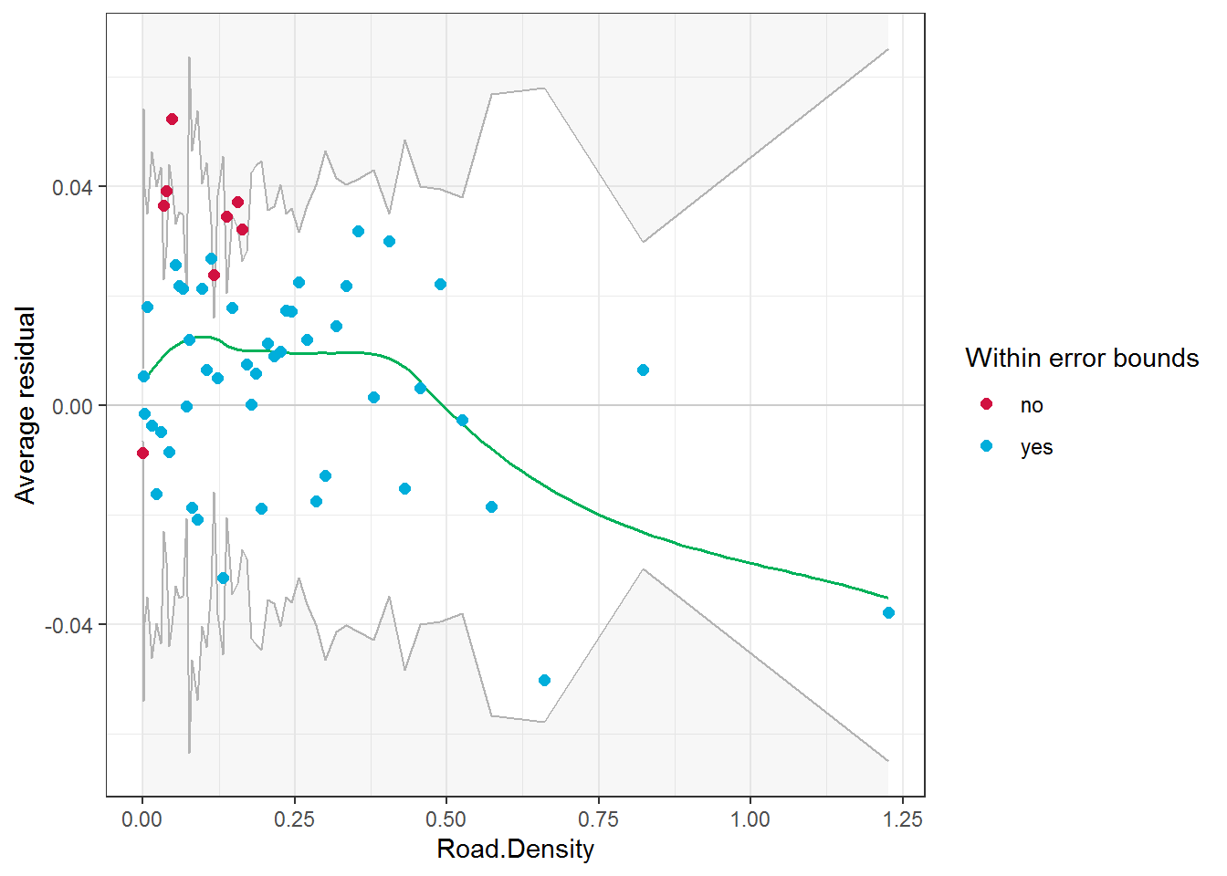
Final notes
The metric that Craig prefers for assessing the quality of a model is a K-fold cross-validation … which is a topic for another primer.
We modelled these data collectively … of course there are seasonal differences that are extremely important, but for illustration purposes the pooling is sufficient, and there are in any case fairly strong signals.
One aspect we have swept under the rug is the serial autocorrealtion in that data. In fact, the
performancepackage has a tool to assess that as well:
check_autocorrelation(rsf.tmb.rs)## Warning: Autocorrelated residuals detected (p = 0.000).It is pretty sure that the autocorrelation (in the residuals) is extremely high. This is not surprising - it is almost guaranteed with movement data. But there is - it seems - a “feeling” that as long as the K-fold validation gives good values, autocorrelation is not something that we need to worry about. There are some tools (in particular: INLA) that will estimate a complex generalized mixed effects model with that serial autocorrelation, but they can be difficult to implement, and computationally quite taxing. Therefore, we’ll just let that topic stay under the rug.
