Organizing the RSF analysis data frame
Resource Selection Functions: Part I
Elie Gurarie
2019-11-29
The Goal: To prepare a data frame for a resource selection analysis that models and eventually predicts habitat use of a subset of woodland caribou against covariates including land cover, road density and elevation.
Background
An RSF quantifies the probability of “used” locations - i.e., places an animal (or, more commonly, animals) have been seen - comared to a set of “available” locations - i.e., places an animal could very well go but wasn’t observed. The RSF does NOT estimate an actual “probability of use”, only a probability with respect to the number of available points that is selected by design. The choice of what is meant by “available” is not trivial, and is closely linked to the questions one is asking, the hypotheses one is testing, and the desired outcomes. We won’t worry too much about these issues here, but will focus on the technical aspects and mechanics of estimating an RSF from movement and landscape data.
The RSF builds directly on spatial analysis that were covered in other primers in this series. Thus, the movement will be the Hay River subset of woodland caribou data, and perform an RSF over the extent of their habitats against several covariates, including EOSD land cover including the fire adjustment, and anthropogenic disturbance.
Note, I refer to previous steps frequently, and link to the relevant sections as needed.
Data organization
There are FOUR major data preparation tasks: (I) Identifying the “used” points, (II) identifying the “available” points, (III) preparing a “stack” of raster layers for relevant covariates and (IV) extracting the covariate values for unifying the used and available locations.
I. Used locations
The used points are collared animal locations, i.e. the movement data. This is just a recap of what we’ve done before, but will get the whole operation rolling.
First, load packages,
pcks <- c("move", "raster", "sf", "ggplot2", "plyr", "scales", "lubridate", "dplyr")
a <- sapply(pcks, require, character = TRUE)
Load the movement data, convert to a simple feature
load("_data/southies.rda") # contains "southies" - the original Movestack
hayriver.sf <- as.data.frame(southies) %>%
  subset(habitat == "Hay River Lowlands" & timestamp < ymd("2012-01-01")) %>%
  st_as_sf(coords = c("location_long", "location_lat"), crs = projection(southies))
Note, it can be helpful to have a LineString (rather than Points) object lying around (see here):
hayriver.lines <- hayriver.sf %>% group_by(nick_name) %>% summarize(do_union=FALSE) %>% st_cast("LINESTRING")For one, we can get a nice quick mapview with the lines:
mapview(hayriver.lines, zcol = "nick_name", map.types = "Esri.WorldPhysical")II. Available locations
The choice of “available” locations is - as mentioned before - not exactly trivial and reflects the kinds of questions you want to answer. We will do something more or less typical, which is characterize the area of use of the population from the movement data with a minimum convex polygon (MCP), and then buffer that polygon with an extra 5 km. This seems like a reasonable approach here.
To compute a buffered MCP, first, make sure that the projection is an (approximately) equidistant projection:
crs(hayriver.sf)## [1] "+proj=longlat +datum=WGS84 +no_defs"This is a long-lat projection, which isn’t terrific. We’ll jump ahead just a little bit and load the EOSD land-cover data, only to extract its projection and assign that to these animals:
eosd <- raster("_data/rasters/EOSD_withfire")
hayriver.sf <- st_transform(hayriver.sf, projection(eosd))
hayriver.lines <- st_transform(hayriver.lines, projection(eosd))
crs(hayriver.sf)
## [1] "+proj=aea +lat_1=50 +lat_2=70 +lat_0=40 +lon_0=-112 +x_0=0 +y_0=0 +ellps=GRS80 +towgs84=0,0,0,0,0,0,0 +units=m +no_defs"Much better - The aea refers to “Albers Equal Area” which is pretty good at small-ish ranges (see this link).
There is an easy to use mcp function in the adehabitatHR package, part of Clément Calenge’s “classic” bundle of ADE packages (stands for Analyses de données ecologique, the HR is “home range”). They do have the slight disadvantage of not working with simple features (yes), but it is easy enough to convert between simple features and spatial points:
require(adehabitatHR)
hayriver.mcp.st <- mcp(as(hayriver.sf, "Spatial"), 100)
plot(hayriver.mcp.st)
plot(hayriver.lines, add = TRUE)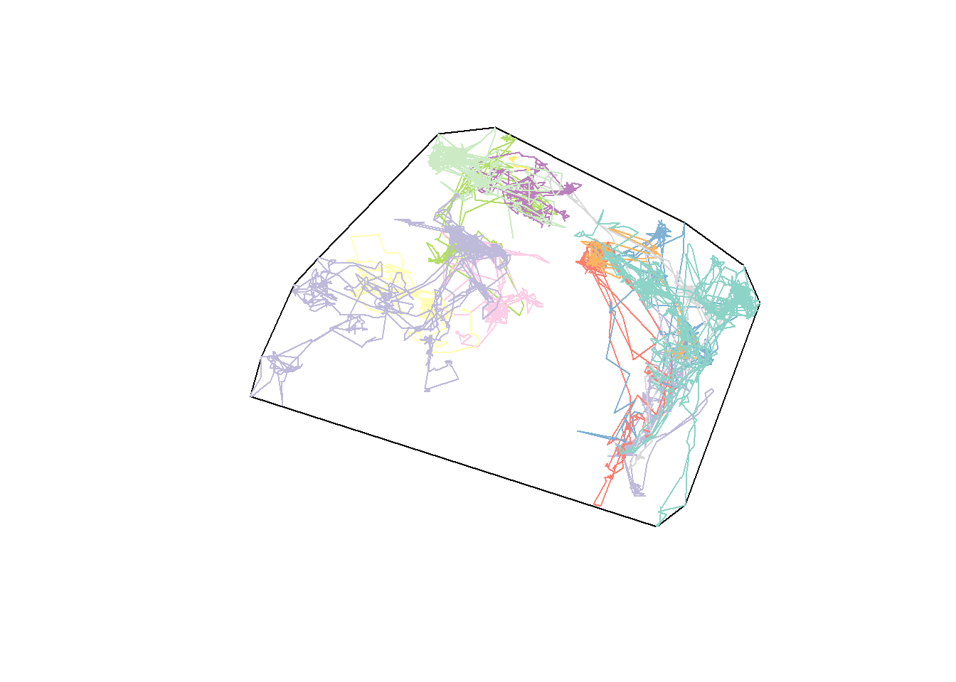
Note, the hayriver.mcp is a spatial object, which needs to be converted to a simple feature for (easy) buffering with st_buffer:
hayriver.mcp <- st_as_sf(hayriver.mcp.st)
hayriver.buffer <- st_buffer(hayriver.mcp, 5e3)
plot(st_geometry(hayriver.buffer), col = "red")
plot(hayriver.mcp, add = TRUE, col = "black")
plot(hayriver.lines, add = TRUE)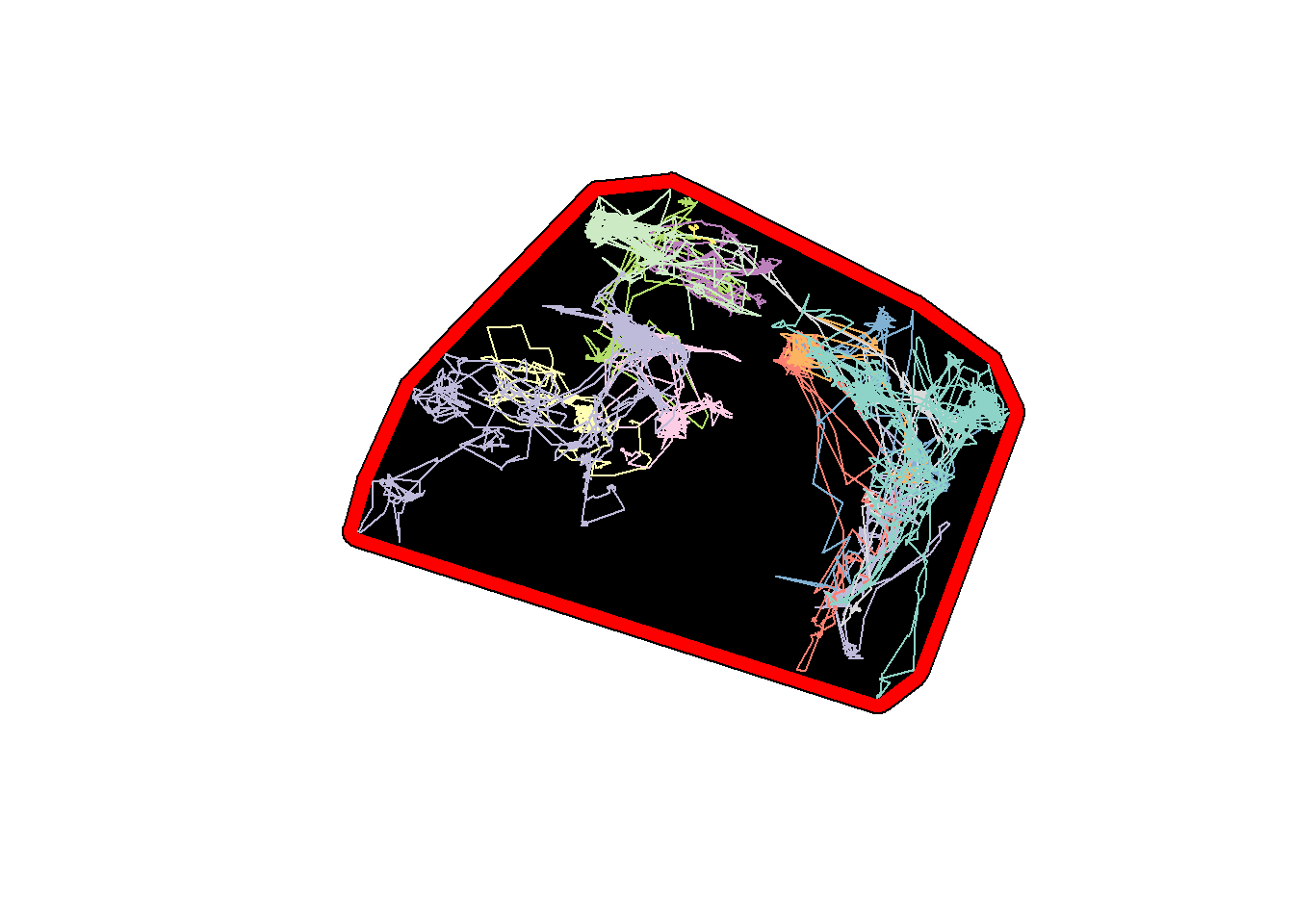
And finally, we sample randomly from the buffered MCP with st_sample(), with a 5 km buffer:
hayriver.avail <- st_sample(hayriver.buffer, 1e3)
plot(st_geometry(hayriver.buffer))
plot(hayriver.avail, add = TRUE, pch = 19, col = alpha("blue", 0.5), cex = 0.5)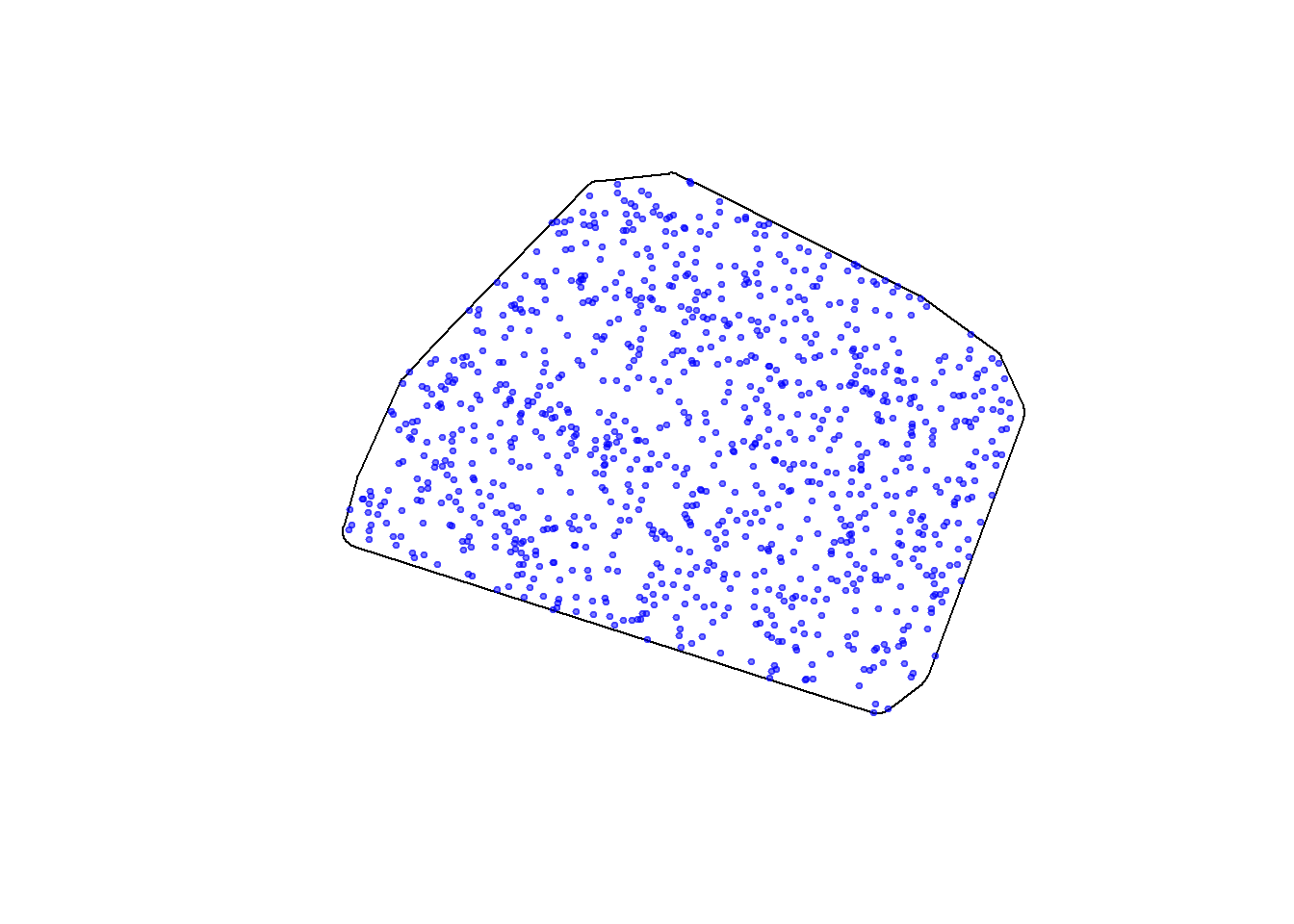
As usual, it is very convenient to make a function that will perform the above steps for a generic set of (simple feature) points used, and an arbitrary buffer distance
sampleFromBufferedMCP <- function(n, used, buffer){
    require(adehabitatHR)
    mcp <- mcp(as(used, "Spatial"), 100) %>% st_as_sf
    mcp.buffered <- st_buffer(mcp, buffer)
    st_sample(mcp.buffered, n)
}
Let’s test this on several subsets of the data (e.g. summer and winter):
hayriver.summer <- subset(hayriver.sf, month(timestamps) %in% c(6,7,8))
hayriver.winter <- subset(hayriver.sf, month(timestamps) %in% c(12,1,2))

summer.avail <- sampleFromBufferedMCP(1e3, hayriver.summer, 5e3)
winter.avail <- sampleFromBufferedMCP(1e3, hayriver.winter, 5e3)

plot(hayriver.mcp.st)
plot(hayriver.buffer, add = TRUE, col = NA, bor = "red")
plot(hayriver.lines, add = TRUE)
plot(summer.avail, add = TRUE, col = alpha("green",.5), cex = 0.5, pch = 19)
plot(winter.avail, add = TRUE, col = alpha("blue",.5), cex = 0.5, pch = 19)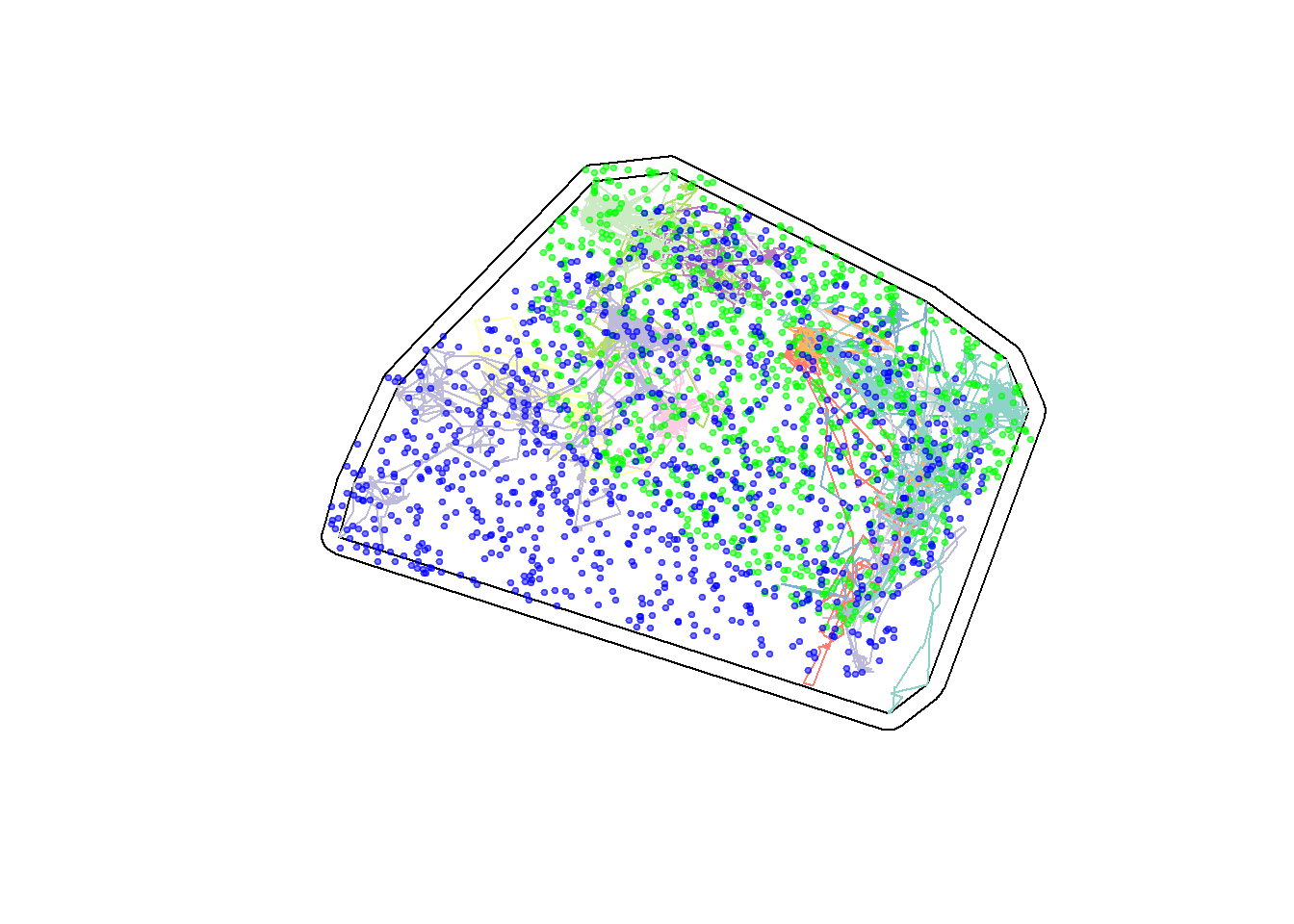
The differences aren’t so large for this subgroup, which is consistent with analyses of seasonal overlap that we performed in the 2018 spatial modeling workshop (see here), where we showed that Buffalo Lake was the only sub-population with a strongly separated seasonal distribution.
III. Combining raster layers
A. EOSD raster - cropped and masked
This is (in my experience) the fussiest step. We’ll start with the fire modified EOSD:
eosd <- raster("_data/rasters/EOSD_withfire")
plot(eosd)
plot(hayriver.lines %>% st_transform(projection(eosd)), add= TRUE) 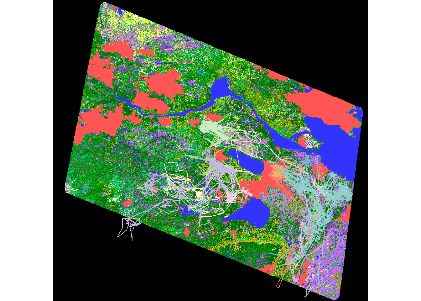
A lot of this data is outside the range of our eventual RSF, so we crop it and mask it to the extent of the movement data.
eosd.cropped <- crop(eosd, as(hayriver.buffer, "Spatial"))
eosd.masked <- mask(eosd.cropped, hayriver.buffer)
plot(eosd.masked)
plot(hayriver.lines %>% st_transform(projection(eosd)), add= TRUE)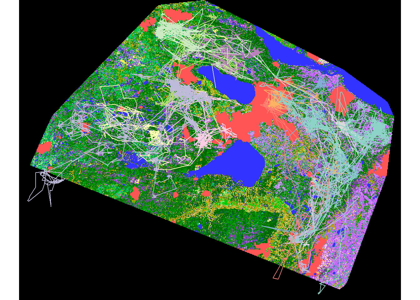
Recall, the details of the raster as as follows:
eosd.masked## class : RasterLayer
## dimensions : 5731, 7297, 41819107 (nrow, ncol, ncell)
## resolution : 30, 30 (x, y)
## extent : -423996.4, -205086.4, 2214172, 2386102 (xmin, xmax, ymin, ymax)
## coord. ref. : +proj=aea +lat_1=50 +lat_2=70 +lat_0=40 +lon_0=-112 +x_0=0 +y_0=0 +datum=NAD83 +units=m +no_defs +ellps=GRS80 +towgs84=0,0,0
## data source : in memory
## names : EOSD_NWT_HRL_clip
## values : 0, 250 (min, max)
## attributes :
## ID OBJECTID Value Description Color Count
## from: 0 1 12 Shadow #333333 365
## to : 19 20 250 Recent Burn #FF5555 6731695i.e.~ it is at a 30m resolution spanning:
(bbox(eosd.masked) %>% apply(1, diff))/1e3## s1 s2
## 218.91 171.93about 220 x 171 km, with about 42 million cells. In other words, it’s LARGE. Eventually - to create a predicitive map - ALL the other raster layers will have to exactly match the resolution and extent of this raster, which means they will have to be LARGE as well.
B. BEAD line density
To get the line densities, we adapt the code from Step 5b to obtain a raster of linear densities. Specifically, we load the linear elements data and compute a “density” of linear elements.
This is, if you recall, a computationally intensive step, but some of the functions we wrote earlier will be useful for this operation. These two functions are getLineDensity and makeLineDensityRaster. The code is included below (click on the button to reveal), and is only slightly modified from the versions here.
getLineDensity():
getLineDensity <- function(pt, lines, r, plotme = FALSE){

  pt.circle <- st_buffer(pt, r)
  intersect <- st_intersection(pt.circle, lines)
  length <- sum(st_length(intersect))/1e3 # in km

  density <- (as.numeric(length)/(pi*(r/1e3)^2)) # in km/km^2

  if(plotme){
    plot(st_geometry(lines))
    plot(pt.circle, add = TRUE, border = 2)
    plot(intersect, add = TRUE, col =3)
  }

  return(density)
}makeLineDensityRaster():
makeLineDensityRaster <- function(lines, resolution, radius){

  require(raster)
  require(doParallel)
  require(magrittr)
  require(sf)
  require(spex)

  # data prep
  density.raster <- raster(extent(lines),
                           resolution = resolution,
                           crs = st_crs(lines))

  print("Getting polygons")

  density.poly <- polygonize(density.raster)
  density.poly.sf <- st_as_sf(density.poly)
  st_crs(density.poly.sf) <- st_crs(lines)

  # buffering lines

  print("Tidying outside of buffer")

  lines.buffered <- st_buffer(lines, radius) %>% st_union
  which.in.buffer <- st_intersection(density.poly.sf, lines.buffered) %>%
    row.names %>% as.numeric

  # cluster prep

  density.poly.list <- split(density.poly.sf[which.in.buffer,], 1:length(which.in.buffer))

  print("Making cluster")

  cl <- makeCluster(detectCores()-1)
  clusterEvalQ(cl, library(sf))
  clusterExport(cl, "getLineDensity")

  print("Computing densities")
  densities.in.buffer <- parSapply(cl, density.poly.list,
                                   getLineDensity, lines = lines, r = radius)
  values(density.raster)[which.in.buffer] <- densities.in.buffer
  density.raster[is.na(density.raster)] <- 0
  stopCluster(cl)

  # check that projection is correct
  projection(density.raster) <- st_crs(lines)
  return(density.raster)
}
A few notes:
makeLineDensityRasteris made significantly faster because it uses paralleliztion … which might not always work within the function as its written (e.g. it may be a bit operating system dependent), in which case the function might need to be unpacked.makeLineDensityRasteralso requires the nesspexpackage, which has a function calledpolygonize()which is a much faster version of therasterToPolygons()function I used in the earlier attempts.
Here, I run this code on the the BEAD.lines data at a 2km distance (which seems, typically, to be relevant for ungulates). Three steps here:
- Load / project / and crop the data to the masked EOSD layer
BEAD.lines <- st_read("_data/BEAD/BEADlines2015_NT1_Bistcho_Calendar_MaxH_Yates_HRL_clip.shp")
BEAD.lines.cropped <- st_crop(BEAD.lines %>% st_transform(projection(eosd.masked)), extent(eosd.masked))- Compute the densities
roadDensity <- makeLineDensityRaster(lines = BEAD.lines.cropped, resolution = 300, 2e3)This is the SLOW step! Make sure you save the resulting raster!
roadDensity <- writeRaster(roadDensity, "_data/RoadDensity")- Match the rasters
Note, we do this to a 300 m resolution (30 m is extremely high for this application!) But, to match the rasters, it is easy enough to increase the resolution via the resample command:
roadDensity.matched <- resample(roadDensity, eosd.masked)This is the KEY function for building layers for an RSF since it makes the layers have the exact same properties (extent, resolution and projection).
To guarantee that this worked, we combine the rasters into an object called a rasterBrick:
## RSF.brick <- brick(eosd.masked, roadDensity.matched)Note, there are two very similar objects “stacks” and “bricks” - craeated and accessed viw the stack() and brick() functions respectively. I am not very clear on the difference between the two, except that bricks are apparently faster - presumably at the cost of retaining some information.
In any case, the brick is a sort of list. Here are all of its properties.
RSF.brick## class : RasterBrick
## dimensions : 5731, 7297, 41819107, 2 (nrow, ncol, ncell, nlayers)
## resolution : 30, 30 (x, y)
## extent : -423996.4, -205086.4, 2214172, 2386102 (xmin, xmax, ymin, ymax)
## coord. ref. : +proj=aea +lat_1=50 +lat_2=70 +lat_0=40 +lon_0=-112 +x_0=0 +y_0=0 +datum=NAD83 +units=m +no_defs +ellps=GRS80 +towgs84=0,0,0
## data source : c:/eli/caribou/NWT/data/RSF_stack.grd
## names : EOSD_NWT_HRL_clip, layer
## min values : 0.0000000, -0.0704177
## max values : 250.000000, 4.586764names(RSF.brick)## [1] "EOSD_NWT_HRL_clip" "layer"And if you want to access a single layer, you can do it my its location in the list:
RSF.brick[[1]]## class : RasterLayer
## band : 1 (of 2 bands)
## dimensions : 5731, 7297, 41819107 (nrow, ncol, ncell)
## resolution : 30, 30 (x, y)
## extent : -423996.4, -205086.4, 2214172, 2386102 (xmin, xmax, ymin, ymax)
## coord. ref. : +proj=aea +lat_1=50 +lat_2=70 +lat_0=40 +lon_0=-112 +x_0=0 +y_0=0 +datum=NAD83 +units=m +no_defs +ellps=GRS80 +towgs84=0,0,0
## data source : c:/eli/caribou/NWT/data/RSF_stack.grd
## names : EOSD_NWT_HRL_clip
## values : 0, 250 (min, max)or by its name:
RSF.brick$EOSD_NWT_HRL_clip## class : RasterLayer
## band : 1 (of 2 bands)
## dimensions : 5731, 7297, 41819107 (nrow, ncol, ncell)
## resolution : 30, 30 (x, y)
## extent : -423996.4, -205086.4, 2214172, 2386102 (xmin, xmax, ymin, ymax)
## coord. ref. : +proj=aea +lat_1=50 +lat_2=70 +lat_0=40 +lon_0=-112 +x_0=0 +y_0=0 +datum=NAD83 +units=m +no_defs +ellps=GRS80 +towgs84=0,0,0
## data source : c:/eli/caribou/NWT/data/RSF_stack.grd
## names : EOSD_NWT_HRL_clip
## values : 0, 250 (min, max)The names are awkward … let’s simplify:
names(RSF.brick) <- c("EOSD", "RoadDensity")And now you can save the brick using the writeRaster command:
writeRaster(RSF.brick, filename = "c:/eli/caribou/NWT/data/RSF_brick_v1.tif")Note: The .tif format is relatively compact (e.g. compared to R’s native .grd format), but this object is still quite large, about 95 MB. So be warned!
As needed, you can then load the raster brick using the brick command:
RSF.brick <- brick("c:/eli/caribou/NWT/data/RSF_brick_v1.tif")C. Digital Elevation Model
Just to make the analysis a little bit more interesting, I also include a digital elevation model. These particular data are from a 30m global elevelation model called “ALOS World 3D (AW3D30)” documentation here. I extracted these data in a relatively tight crop around the Hay River Lowlands at 100 m resolution (for tractability).
Note: I tried obtaining 30m resolution data from the new and much vaunted Arctic DEM - but there was really too much missing information, possibly because this study area is really a the edge of the Arctic DEM’s coverage.
Here are the raw DEM data:
DEM <- raster("_data/HayRiverDEM_100m.tif")
plot(DEM)
contour(DEM, add = TRUE, nlevels = 20)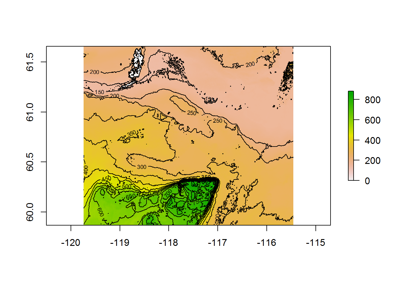
Always fun (and easy) to layer these on top of a mapview:
mapview(DEM, map.types = "Esri.WorldImagery")There isn’t too much going on here. Aside from Great Slave Lake to the northeast, there is a relatively high (600-800 m) plateau jutting in from the south.
Matching this raster to our brick is straightforward. But note: it is faster to first reproject this raster at a coarse resolution (e.g. the approximate native 100 m) and THEN resample to match the brick, rather than directly project this to. In other words, this:
DEM.matched <- projectRaster(DEM, RSF.brick)is VERY slow. But this:
DEM.projected <- projectRaster(DEM, crs = projection(RSF.brick), res = 100)
DEM.matched <- resample(DEM.projected, RSF.brick)
is reasonable. We can add this layer to our final brick:
RSF.brick[[3]] <- DEM.matched
names(RSF.brick) <- c("EOSD", "RoadDensity", "DEM")
writeRaster(RSF.brick,
            filename = "c:/eli/caribou/NWT/data/RSF_brick_v2.tif")
IV. Generating final data frame
Load the saved brick of environmental covariates :
RSF.brick <- brick("c:/eli/caribou/NWT/data/RSF_brick_v2.tif")When you save the raster brick as a GeoTIFF (.tif) - you lose the names. To retain them, you need to save it in the native (uncompressed) format. This is quite large, so we’ll stick to .tifs and rename the levels as needed. You also lose the definitions of the levels for the categorical variable, but at this stage that is not very important.
names(RSF.brick) <- c("EOSD", "Road Density", "DEM")By default, all layers are plotted (using a crop here for tractability):
RSF.brick.small <- crop(RSF.brick,
                        extent(c(-2.6e5,-2.1e5, 22.5e5, 23e5)))
plot(RSF.brick.small, nc = 3)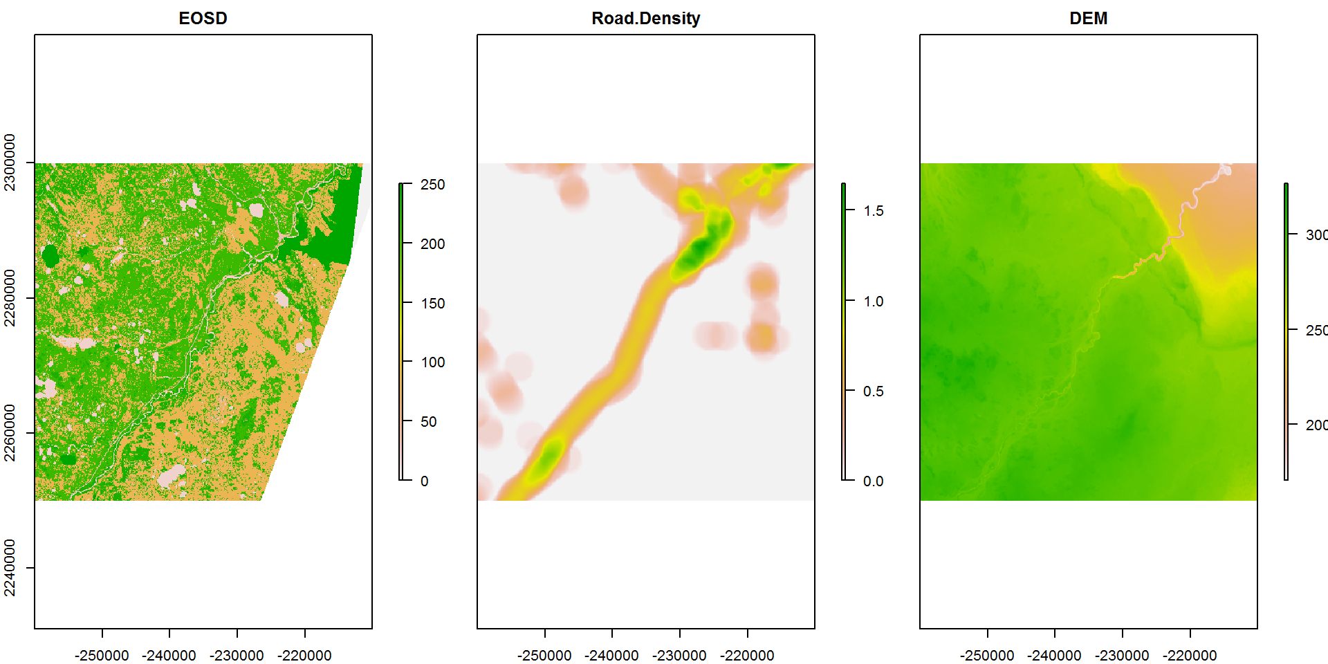
Most importantly, the extract function slices through all the layers at once. Here, for example, are the values of all three layers for the first six locations of the Hay River data
extract(RSF.brick.small, head(hayriver.sf))## EOSD Road.Density DEM
## [1,] 211 0.00000000 300.7350
## [2,] 82 0.21480259 301.5301
## [3,] 81 0.04745031 308.1896
## [4,] 212 0.18918139 303.9097
## [5,] 211 0.00000000 295.7391
## [6,] 81 0.03215680 296.6236It is now easy to build the RSF data frame. The complete set of USED covariates is simply
Covars.used <- extract(RSF.brick, hayriver.sf)And the AVAILABLE covariates are:
Covars.avail <- extract(RSF.brick, st_coordinates(hayriver.avail))We combine these two together, but it would be good to retain information about the time and ID of the individuals in a final data base. The rbind.fill function in plyr stacks data frames with similar, but not exactly identical, column names, and fills the empty gaps with NA.
hayriver.used.df <- hayriver.sf[,c("nick_name", "timestamp")] %>% cbind(st_coordinates(hayriver.sf), Covars.used, Used = TRUE)
hayriver.RSF <- rbind.fill(hayriver.used.df, data.frame(Covars.avail, Used = FALSE))
Our data frame is almost ready, it looks like this:
str(hayriver.RSF)## 'data.frame': 9908 obs. of 9 variables:
## $ nick_name : Factor w/ 201 levels "BI318","BI319",..: 63 63 63 63 63 63 63 63 63 63 ...
## $ timestamp : chr "2007-02-22 22:30:00" "2007-02-25 22:13:00" "2007-02-28 22:58:00" "2007-03-03 21:45:00" ...
## $ geometry : chr "c(-258895.210792302, 2255297.96131929)" "c(-255314.918559923, 2265023.81882329)" "c(-253799.721722459, 2267979.39271626)" "c(-257246.920353896, 2264706.02814558)" ...
## $ X : num -258895 -255315 -253800 -257247 -252508 ...
## $ Y : num 2255298 2265024 2267979 2264706 2262221 ...
## $ EOSD : num 211 82 81 212 211 81 82 83 212 83 ...
## $ Road.Density: num 0 0.2148 0.0475 0.1892 0 ...
## $ DEM : num 301 302 308 304 296 ...
## $ Used : logi TRUE TRUE TRUE TRUE TRUE TRUE ...Final tidying
Just a few more items for final data prep.
We probably don’t need the geometry column (that’s a vestige of its sf origins, and the coordinates themselves are in the X and Y columns), but it might be nice to have the lat-long coordinates. The following code is a bit fussy (due to some simple feature weirdness) but ultimately returns a column of lat/long:
ll <- hayriver.RSF$geometry %>% st_sfc %>% st_transform(4326) %>% st_coordinates %>% data.frame %>% plyr::rename(c(X = "longitude", Y = "latitude"))
hayriver.RSF <- cbind(hayriver.RSF, ll) %>% mutate(geometry = NULL)
It would be very convenient to have a column of EOSD land layers by name. Recall that they are stored in the EOSD raster levels:
levels(eosd)## [[1]]
## ID OBJECTID Value Description Color Count
## 1 0 1 12 Shadow #333333 365
## 2 1 2 20 Water #3333FF 5559064
## 3 2 3 32 Rock/Rubble #CCCCCC 67
## 4 3 4 33 Exposed/Barren Land #996633 13635
## 5 4 5 34 Developed #CC6699 64239
## 6 5 6 40 Bryoids #FFCCFF 96789
## 7 6 7 51 Shrub Tall #FFFF33 72952
## 8 7 8 52 Shrub Low #FFFF99 668629
## 9 8 9 81 Wetland-treed #9933CC 2358766
## 10 9 10 82 Wetland-shrub #CC66FF 4242600
## 11 10 11 83 Wetland-herb #CC99FF 1160373
## 12 11 12 100 Herbs #CCFF33 514846
## 13 12 13 211 Coniferous-dense #006600 6715586
## 14 13 14 212 Coniferous-open #009900 11162064
## 15 14 15 213 Coniferous-sparse #00CC66 3236051
## 16 15 16 221 Broadleaf-dense #00CC00 917321
## 17 16 17 222 Broadleaf-open #99FF99 985631
## 18 17 18 231 Mixedwood-dense #CC9900 3088338
## 19 18 19 232 Mixedwood-open #CCCC66 600763
## 20 19 20 250 Recent Burn #FF5555 6731695We need to match our EOSD column to the Value column of this object, and extract the Description. We do that (in one line) by merging and renaming:
hayriver.RSF <- merge(hayriver.RSF, levels(eosd)[[1]][,c("Value","Description")], by.x = "EOSD", by.y = "Value") %>% plyr::rename(c(Description = "EOSD.class")) Here’s a useful quick survey of the landscape data:
with(hayriver.RSF, table(EOSD.class, Used))## Used
## EOSD.class FALSE TRUE
## Broadleaf-dense 7 3
## Broadleaf-open 6 6
## Bryoids 3 3
## Coniferous-dense 161 1373
## Coniferous-open 217 3174
## Coniferous-sparse 40 460
## Developed 3 0
## Exposed/Barren Land 0 0
## Herbs 0 0
## Mixedwood-dense 55 164
## Mixedwood-open 12 72
## Recent Burn 72 650
## Rock/Rubble 0 0
## Shadow 0 0
## Shrub Low 4 32
## Shrub Tall 1 0
## Water 91 91
## Wetland-herb 25 682
## Wetland-shrub 105 1404
## Wetland-treed 53 724Also - the nick_name is still retaining all 201 levels of the original data frame. Lets drop those unused levels:
hayriver.RSF$nick_name <- droplevels(hayriver.RSF$nick_name)Finally, often this processing shuffles the order of the data. It would be good to sort the data, by ID and by time, so that they are ordered in a reasonable way:
hayriver.RSF <- arrange(hayriver.RSF, nick_name, timestamp)Finally, be sure to save this data frame:
save(hayriver.RSF, file = "_data/hayriver_RSF.rda")Complete code
Click below to show complete code from this document.
## output:
##   html_document:
##     code_folding: hide
knitr::opts_chunk$set(echo = TRUE, cache=TRUE, message = FALSE, warning = FALSE)
## setwd("C:/Users/Elie/box sync/caribou/NWT/RSF/primers")
pcks <- c("move", "raster", "sf", "ggplot2", "plyr", "scales", "lubridate", "dplyr")
a <- sapply(pcks, require, character = TRUE)
load("_data/southies.rda") # contains "southies" - the original Movestack
hayriver.sf <- as.data.frame(southies) %>%
  subset(habitat == "Hay River Lowlands" & timestamp < ymd("2012-01-01")) %>%
  st_as_sf(coords = c("location_long", "location_lat"), crs = projection(southies))
hayriver.lines <- hayriver.sf %>% group_by(nick_name) %>% summarize(do_union=FALSE) %>% st_cast("LINESTRING")
require(mapview)
mapview(hayriver.lines, zcol = "nick_name", map.types = "Esri.WorldPhysical")
crs(hayriver.sf)
eosd <- raster("_data/rasters/EOSD_withfire")
hayriver.sf <- st_transform(hayriver.sf, projection(eosd))
hayriver.lines <- st_transform(hayriver.lines, projection(eosd))
crs(hayriver.sf)
require(adehabitatHR)
hayriver.mcp.st <- mcp(as(hayriver.sf, "Spatial"), 100)
plot(hayriver.mcp.st)
plot(hayriver.lines, add = TRUE)
hayriver.mcp <- st_as_sf(hayriver.mcp.st)
hayriver.buffer <- st_buffer(hayriver.mcp, 5e3)
plot(st_geometry(hayriver.buffer), col = "red")
plot(hayriver.mcp, add = TRUE, col = "black")
plot(hayriver.lines, add = TRUE)
hayriver.avail <- st_sample(hayriver.buffer, 1e3)
plot(st_geometry(hayriver.buffer))
plot(hayriver.avail, add = TRUE, pch = 19, col = alpha("blue", 0.5), cex = 0.5)
sampleFromBufferedMCP <- function(n, used, buffer){
    require(adehabitatHR)
    mcp <- mcp(as(used, "Spatial"), 100) %>% st_as_sf
    mcp.buffered <- st_buffer(mcp, buffer)
    st_sample(mcp.buffered, n)
}
hayriver.summer <- subset(hayriver.sf, month(timestamps) %in% c(6,7,8))
hayriver.winter <- subset(hayriver.sf, month(timestamps) %in% c(12,1,2))

summer.avail <- sampleFromBufferedMCP(1e3, hayriver.summer, 5e3)
winter.avail <- sampleFromBufferedMCP(1e3, hayriver.winter, 5e3)

plot(hayriver.mcp.st)
plot(hayriver.buffer, add = TRUE, col = NA, bor = "red")
plot(hayriver.lines, add = TRUE)
plot(summer.avail, add = TRUE, col = alpha("green",.5), cex = 0.5, pch = 19)
plot(winter.avail, add = TRUE, col = alpha("blue",.5), cex = 0.5, pch = 19)
eosd <- raster("_data/rasters/EOSD_withfire")
plot(eosd)
plot(hayriver.lines %>% st_transform(projection(eosd)), add= TRUE)
eosd.cropped <- crop(eosd, as(hayriver.buffer, "Spatial"))
eosd.masked <- mask(eosd.cropped, hayriver.buffer)
plot(eosd.masked)
plot(hayriver.lines %>% st_transform(projection(eosd)), add= TRUE)
eosd.masked
(bbox(eosd.masked) %>% apply(1, diff))/1e3
## getLineDensity <- function(pt, lines, r, plotme = FALSE){
##
##   pt.circle <- st_buffer(pt, r)
##   intersect <- st_intersection(pt.circle, lines)
##   length <- sum(st_length(intersect))/1e3 # in km
##
##   density <- (as.numeric(length)/(pi*(r/1e3)^2)) # in km/km^2
##
##   if(plotme){
##     plot(st_geometry(lines))
##     plot(pt.circle, add = TRUE, border = 2)
##     plot(intersect, add = TRUE, col =3)
##   }
##
##   return(density)
## }
## makeLineDensityRaster <- function(lines, resolution, radius){
##
##   require(raster)
##   require(doParallel)
##   require(magrittr)
##   require(sf)
##   require(spex)
##
##   # data prep
##   density.raster <- raster(extent(lines),
##                            resolution = resolution,
##                            crs = st_crs(lines))
##
##   print("Getting polygons")
##
##   density.poly <- polygonize(density.raster)
##   density.poly.sf <- st_as_sf(density.poly)
##   st_crs(density.poly.sf) <- st_crs(lines)
##
##   # buffering lines
##
##   print("Tidying outside of buffer")
##
##   lines.buffered <- st_buffer(lines, radius) %>% st_union
##   which.in.buffer <- st_intersection(density.poly.sf, lines.buffered) %>%
##     row.names %>% as.numeric
##
##   # cluster prep
##
##   density.poly.list <- split(density.poly.sf[which.in.buffer,], 1:length(which.in.buffer))
##
##   print("Making cluster")
##
##   cl <- makeCluster(detectCores()-1)
##   clusterEvalQ(cl, library(sf))
##   clusterExport(cl, "getLineDensity")
##
##   print("Computing densities")
##   densities.in.buffer <- parSapply(cl, density.poly.list,
##                                    getLineDensity, lines = lines, r = radius)
##   values(density.raster)[which.in.buffer] <- densities.in.buffer
##   density.raster[is.na(density.raster)] <- 0
##   stopCluster(cl)
##
##   # check that projection is correct
##   projection(density.raster) <- st_crs(lines)
##   return(density.raster)
## }
##
##
## BEAD.lines <- st_read("_data/BEAD/BEADlines2015_NT1_Bistcho_Calendar_MaxH_Yates_HRL_clip.shp")
## BEAD.lines.cropped <- st_crop(BEAD.lines %>% st_transform(projection(eosd.masked)), extent(eosd.masked))
## roadDensity <- makeLineDensityRaster(lines = BEAD.lines.cropped, resolution = 300, 2e3)
## roadDensity <- writeRaster(roadDensity, "_data/RoadDensity")
roadDensity <- raster("_data/RoadDensity")
## roadDensity.matched <- resample(roadDensity, eosd.masked)
RSF.brick <- brick(eosd.masked, roadDensity.matched)
RSF.brick <- brick("c:/eli/caribou/NWT/data/RSF_stack")
RSF.brick
names(RSF.brick)
RSF.brick[[1]]
RSF.brick$EOSD_NWT_HRL_clip
names(RSF.brick) <- c("EOSD", "RoadDensity")
## writeRaster(RSF.brick, filename = "c:/eli/caribou/NWT/data/RSF_brick_v1.tif")
RSF.brick <- brick("c:/eli/caribou/NWT/data/RSF_brick_v1.tif")
DEM <- raster("_data/HayRiverDEM_100m.tif")
plot(DEM)
contour(DEM, add = TRUE, nlevels = 20)
require(mapview); DEM <- raster("_data/HayRiverDEM_100m.tif")
mapview(DEM, map.types = "Esri.WorldImagery")
## DEM.matched <- projectRaster(DEM, RSF.brick)
## DEM.projected <- projectRaster(DEM, crs = projection(RSF.brick), res = 100)
## DEM.matched <- resample(DEM.projected, RSF.brick)
## RSF.brick[[3]] <- DEM.matched
## names(RSF.brick) <- c("EOSD", "RoadDensity", "DEM")
## writeRaster(RSF.brick,
##             filename = "c:/eli/caribou/NWT/data/RSF_brick_v2.tif")
RSF.brick <- brick("c:/eli/caribou/NWT/data/RSF_brick_v2.tif")
names(RSF.brick) <- c("EOSD", "Road Density", "DEM")
RSF.brick.small <- crop(RSF.brick,
                        extent(c(-2.6e5,-2.1e5, 22.5e5, 23e5)))
plot(RSF.brick.small, nc = 3)
extract(RSF.brick.small, head(hayriver.sf))
Covars.used <- extract(RSF.brick, hayriver.sf)
Covars.avail <- extract(RSF.brick, st_coordinates(hayriver.avail))
hayriver.used.df <- hayriver.sf[,c("nick_name", "timestamp")] %>% cbind(st_coordinates(hayriver.sf), Covars.used, Used = TRUE)
hayriver.RSF <- rbind.fill(hayriver.used.df, data.frame(Covars.avail, Used = FALSE))
str(hayriver.RSF)
ll <- hayriver.RSF$geometry %>% st_sfc %>% st_transform(4326) %>% st_coordinates %>% data.frame %>% plyr::rename(c(X = "longitude", Y = "latitude"))
hayriver.RSF <- cbind(hayriver.RSF, ll) %>% mutate(geometry = NULL)
levels(eosd)
hayriver.RSF <- merge(hayriver.RSF, levels(eosd)[[1]][,c("Value","Description")], by.x = "EOSD", by.y = "Value") %>% plyr::rename(c(Description = "EOSD.class"))
with(hayriver.RSF, table(EOSD.class, Used))
hayriver.RSF$nick_name <- droplevels(hayriver.RSF$nick_name)
hayriver.RSF <- arrange(hayriver.RSF, nick_name, timestamp)
## save(hayriver.RSF, file = "_data/hayriver_RSF.rda")
f <- "Step06_RSF_PartI"
require(knitr); require(rmarkdown)
# purl(paste0(f, ".Rmd"), output = paste0("_code/",f,".r"), documentation = 0)
render_site(paste0(f, ".Rmd"))
nlines <- length(readLines(paste0("_code/",f,".r")))
## NA