Experimental measurements are never perfect, even with
sophisticated modern instruments. Two main types or measurement
errors are recognized: (a) systematic error, in which
every measurement is consistently less than or greater than
the correct value by a certain percentage or amount, and (b)
random error, in which there are unpredictable variations
in the measured signal from moment to moment or from measurement
to measurement. This latter type of error is often called noise,
by analogy to acoustic noise. There are
many sources of noise in physical measurements, such as building
vibrations, air currents, electric power fluctuations, stray
radiation from nearby electrical equipment, static electricity,
interference from radio and TV transmissions, turbulence in the
flow of gases or liquids, random thermal motion of molecules,
background radiation from natural radioactive elements, "cosmic
rays" from outer space (seriously), the basic quantum nature of
matter and energy itself ,
and digitization
noise (the rounding of numbers to a fixed number of
digits). Then of course these is the
ever-present "human error", which can be a major factor anytime
humans are involved in operating, adjusting, recording,
calibrating, or controlling instruments and in preparing samples
for measurement. If random error is present, then a set of repeat
measurements will yield results that are not all the same but
rather vary or scatter around some average value,
which is the sum of the values divided by
the number of data values "d", given by sum(d)./length(d) in
Matlab/Octave notation, or simply mean(d). The most common
way to measure the amount of variation or dispersion of a set of
data values is to compute the standard
deviation, "std", which is the square root of the sum of the
squares of the deviations from the average divided by one less
that the number of data points:
sqrt(sum((d-mean(d)).^2)./(length(d)-1)) or, in Matlab/Octave
notation, simply std(d). A basic fact of random variables is that
when they combine, the results must be calculated statistically.
For example, when two random variables are added, the standard
deviation of the sum is the "quadratic sum" (the square root of
the sum of the squares) of the standard deviations of the
individual variables, as demonstrated by this simple experiment.
In Matlab, the function "randn(1,n)" returns n random numbers with
a standard deviation that approaches 1 for large n. Therefore:
and
The term "signal" actually has two meanings: in the more
general sense, it can mean the entire data recording,
including the noise and other artifacts, as in the "raw signal"
before processing is applied. But it it can also mean only the desirable
or important part of the data, the true
underlying signal that you seek to measure, as in
"signal-to-noise ratio". A fundamental problem in signal
measurement is distinguishing the true underlying signal from the
noise. You might want to measure the average of the signal over a
certain time period or the height of a peak or the area under a
peak that occurs in the data. For example, in the absorption
spectrum in the right-hand half of Figure 1 in the previous
section, the "important" parts of the data are probably the
absorption peaks located at 520 and 550 nm. The height or the
position of either of those peaks might be considered
the signal, depending on the application. In this example,
the height of the largest peak is about 0.08 absorbance units. But
how to measure the noise?
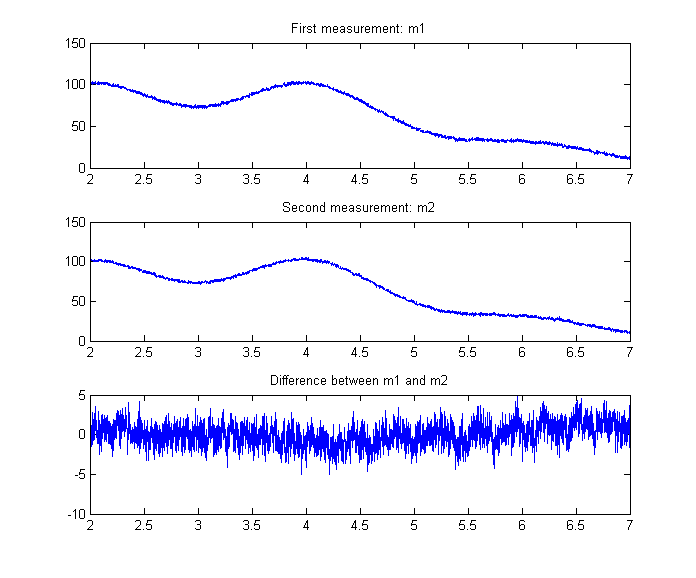
If you are lucky enough to have a sample and an instrument that
are completely stable (except for the random noise), an
easy way to isolate and measure the noise is to record two
signals m1 and m2 under the same conditions, subtract them
point-by-point. Then the standard
deviation of the noise in the original signals
is not std(m1-m2) as you might think (that gives too high a
value), but rather sqrt((std(m1-m2)2)/2),
as shown by a simple
derivation based on the rules
for mathematical error propagation. The process is
demonstrated quantitatively and graphically by the
Matlab/Octave script SubtractTwoMeasurements.m
(Graphic).
But what if the measurements are not that reproducible or that you
had only one recording
of that spectrum and no other data? In that case, you could
try to estimate the noise in that single recording, based on the assumption
that the visible short-term fluctuations in the signal
- the little random wiggles superimposed on the smooth signal -
are noise and not part of the true underlying signal. That depends
on some knowledge of the origin of the signal and the possible
forms it might take. The examples in previous section are
absorption spectra of liquid solutions over the wavelength range
of 450 nm to 700 nm, which ordinarily exhibit broad smooth peaks
with a width of the order of 10 to 100 nm, so the little wiggles
must be noise. In this case, those fluctuations amount to a
standard deviation of about 0.001. Often the best way to
measure the noise is to locate a section of the signal on the
baseline where the signal is flat and to compute the standard
deviation in that section. This is easy to do with a computer if
the signal is digitized. The important
thing is that you must know enough about the measurement and
the data it generates to recognize the kind of signals that is
is likely to generate, so you have some hope of knowing what
is signal and what is noise.
It's important to appreciate that the standard
deviations calculated of a small set of measurements can be much
higher or much lower than the actual standard deviation of a
larger number of measurements. For example, the Matlab/Octave
function randn(1,n), where n is an integer, returns
n random numbers that have on average a mean of
zero and a standard deviation of 1.00 if n is large. But
if n is small, however, standard deviations will be
different each time you evaluate that function; for example if
n=5, randn(1,5), the standard
deviations might vary randomly from 0.5 to 2 or even more. The is
the unavoidable nature of small sets of random numbers: the
standard deviation calculated from a small set of numbers is only
a very rough approximation to the real underlying standard
deviation.
A quick but approximate way to estimate the amplitude of noise
visually is the peak-to-peak range, which is the
difference between the highest and the lowest values in a region
where the signal is flat. The ratio of peak-to-peak
range of n=100 normally-distributed random numbers to its
standard deviation is approximately 5, as can be proved by running
this line of Matlab/Octave code several times:
n=100;rn=randn(1,n);(max(rn)-min(rn))/std(rn). For
example, the data on the right half of the figure below, has a
peak in the center with a height of about 1.0. The
peak-to-peak noise on the baseline is also about 1.0, so the
standard deviation of the noise is about 1/5th of that, or 0.2.However,
that ratio varies with the logarithm of n and is closer to
3 when n = 10 and to 9 when n = 100000. In
contrast, the standard deviation becomes closer and closer to the
true value as n increases. It's better to compute the
standard deviation if possible.
In addition to the standard deviation, it's also possible
to measure the mean absolute deviation ("mad"). The
standard deviation is larger than the mean absolute deviation
because the standard deviation weights the large deviation more
heavily. For a normally-distributed random variable, the mean
absolute deviation is on average 80% of the standard deviation:
mad=0.8*std.
The quality
of a signal is often expressed quantitatively as the
signal-to-noise ratio (S/N ratio), which is the ratio of
the true underlying signal amplitude (e.g. the average amplitude
or the peak height) to the standard deviation of the noise. Thus
the S/N ratio of the spectrum in Figure 1 is about 0.08/0.001 =
80, and the signal in Figure 3 has a S/N ratio of 1.0/0.2
= 5. So we would say that the quality of the signal in
Figure 1 is better than that in Figure 3 because it has a
greater S/N ratio. Measuring the S/N ratio is much easier
if the noise can be measured separately, in the absence of
signal. Depending on the type of experiment, it may be possible
to acquire readings of the noise alone, for example on a segment
of the baseline before or after the occurrence of the signal.
However, if the magnitude of the noise depends on the level of
the signal, then the experimenter must try to produce a constant
signal level to allow measurement of the noise on the signal. In
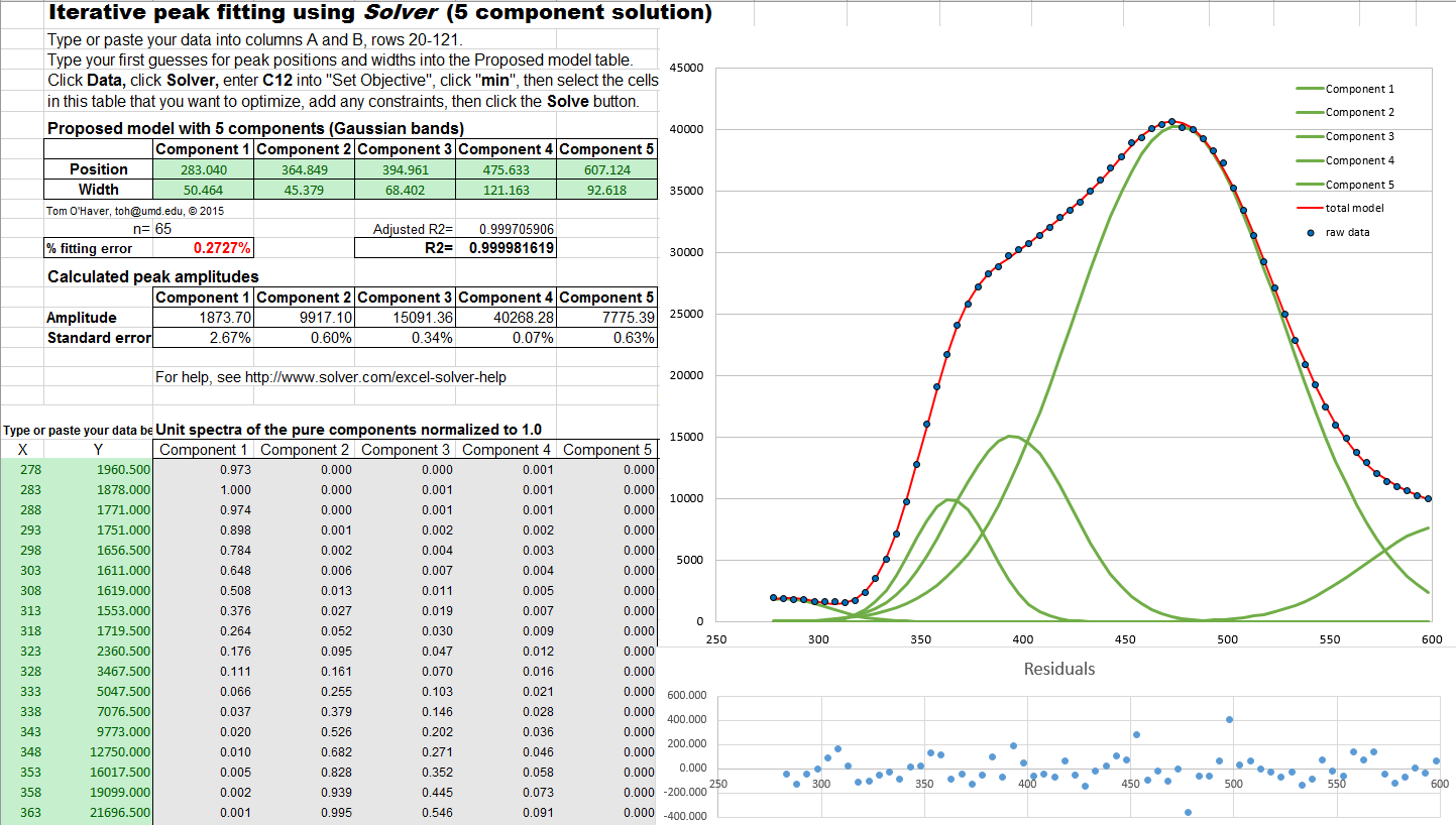
some cases, where you can model the shape of the signal
accurately by means of a mathematical function (such as a polynomial or the weighted sum
of a number of peak shape
functions), the noise may be isolated by subtracting the model
from the unsmoothed experimental signal, for example by looking
at the residuals in least-squares curve fitting, as in this example. If
possible, it's usually better to determine the standard
deviation of repeated measurements of the thing that you want to
measure (e.g. the peak heights or areas), rather than trying to
estimate the noise from a single recording of the data.
Detection limit. The
"detection limit" is defined as the smallest signal that you can
reliably detect in the presence of noise. In quantitative
analysis, it is usually
defined as the concentration that produces the smallest
detectable signal (Reference
90). A signal below the detection limit cannot be reliably
detected, that is, if the measurement is repeated, the signal
will often be "lost in the noise" and reported as zero. A signal
above the detection limit will be reliable detected and will
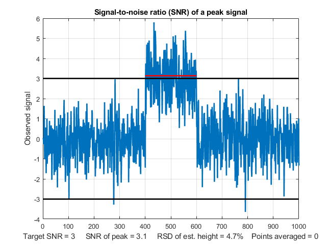
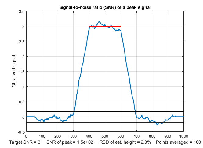
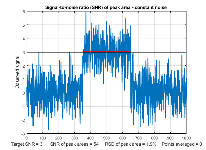
seldom or never reported as zero. The most common definition of
signal-to-noise ratio at the detection limit is 3. This is
illustrated in the figure on the left (created by the
Matlab/Octave script SNRdemo.m). This
shows a noisy signal in the form of a rectangular pulse. We
define the "signal" as the average signal magnitude during the
pulse, indicated by the red line, which is 3 ("signal" in line 3
of the script, which you can change). We define the "noise" as
the the standard deviation of the random noise on the baseline
before and after the pulse, which is about 1.0 (roughly 1/5 of
the peak-to-peak baseline noise indicated by the two black
horizontal lines). So the signal-to-noise ratio (SNR) in this
case is about 3, which is the most common definition of
detection limit. This means that this is the lowest signal that
can be reliably detected and that signals lower than this should
be reported as "undetectable".
But there is a problem. This signal is clearly detectable by
eye; in fact, it would be possible to visually detect lower
signals than this. How can this be? The answer is "averaging".
When you look at this signal, you are unconsciously
estimating the average of the data points on the signal
pulse and on the base-line, and your visual detection ability in
enhanced by this averaging. Without that averaging, looking only
at individual data points in the signal, only about
half those individual points would meet the SNR=3 criterion. You
can see in the graphic above that several points on the signal
peak are actually lower that some of the data points on
the baseline. But this is not a problem in practice, because any
properly written software will include averaging that duplicates
the visual averaging that we all do.
In the script SNRdemo.m, the number of
points averaged is controlled by the variable "AveragePoints" in
line 7. If you set that to 5, the resulting graphic (below on
the left) shows that all of the signal
points are above the highest baseline points. This graphic more
accurately represents what we judge when we look at a signal
like that in the previous graphic: a clear separation of signal
and baseline. The SNR of the peak has improved from 3.1 to 7.7
and the detection limit will be correspondingly reduced.
As a rule of thumb, the noise decreases by the roughly the
square root of the number of points averaged (sqrt(5)=2.2).
Higher values will further improve the SNR and reduce the
relative standard deviation of the average signal, but the
response time - which is the time it takes for the signal to
reach the average value - will become slower and slower as the
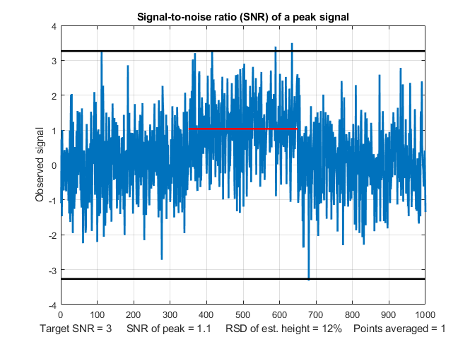
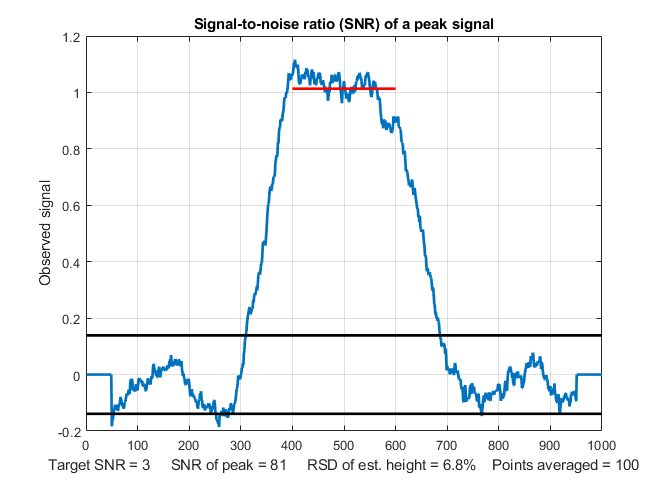
number of points averaged increases. This is shown by this graphic with 100 points
averaged. With a much lower signal, where the SNR is only 1.0,
the raw signal is barely detectable
visually, but with a 100 point average, the signal precision is good.
Digital averaging beats visual averaging in this case.
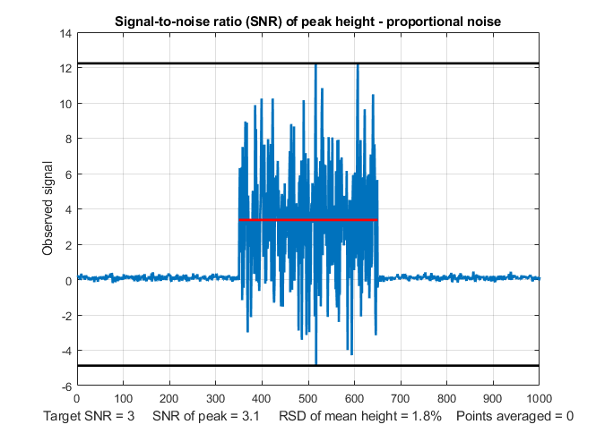
In SNRdemo.m, the noise is constant
and independent of the signal amplitude. In the variant SNRdemoHetero.m, the noise in the
signal is directly proportional to the signal level, and as a
result the detection limit depends on the constant baseline
noise (graphic). In the variant
SNRdemoArea.m, it is the peak area
that is measured rather than the peak height, and as a
result the SNR is improved by the square root of the width of
the peak (graphic). An example of a practical application of
a signal like this would be to turn on a warning light or buzzer
if the signal ever exceeds a threshold value of 1.5 volts, for
the signal illustrated in the figures above. This would not work
if you used the raw unaveraged signal in the first figure; there
is no threshold value that would never be exceeded by the
baseline but always exceeded by the signal. Only the
averaged signal would reliably turn on the alarm above
the threshold and never activate it below the threshold.
You will also hear the term "Limit of determination", which
is the lowest signal or concentration that achieves a minimum
acceptable precision, defined as the relative standard deviation
of the signal amplitude. That is defined at much higher
signal-to-noise ratio, say 10 or 20, depending on the
requirements of your applications.
Averaging such as done here is the simplest form of
"smoothing", which is covered in the next chapter.
Ensemble averaging.
One key thing that really distinguishes signal from noise is
that random noise is not the same from one measurement of the
signal to the next, whereas the genuine signal is at least
partially reproducible. So if the signal can be measured more
than once, use can be made of this fact by measuring the signal
over and over again, as fast as is practical, and adding up all the
measurements point-by-point, then dividing by the number of
signals averaged. This is called ensemble averaging,
also called "ensemble averaging", and it is one of the most
powerful methods for improving signals, when it can be applied.
For this to work properly, the noise must be random and the
signal must occur at the same time in each repeat.
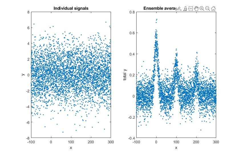
Window 1 (left) is a single measurement of a very noisy
signal. There is actually a broad peak near the center of this
signal, but it is difficult to measure its position, width,
and height accurately because the S/N ratio is very poor.
Window 2 (right) is the average of 9 repeated measurements of
this signal, clearly showing the peak emerging from the noise.
The expected improvement in S/N ratio is 3 (the square root of
9). Often it is possible to average hundreds
of measurements, resulting in much more substantial
improvement. The S/N ratio in the resulting average signal in
this example is about 5.
The Matlab/Octave script EnsembleAverageDemo.m
demonstrates the technique graphically; click for graphic. Another
example is shown in the video animation (EnsembleAverage1.wmv or EnsembleAverageDemo.gif)
which shows the ensemble averaging of 1000 repeats of a signal,
improving the S/N ratio by about 30 times. (Digitization
noise can also be reduced by ensemble averaging, but only if
small amounts of random noise are present in, or added to,
the signal;
see Appendix I).
Frequency distribution.
Sometimes the signal and the noise can be partly distinguished on
the basis of frequency components:
for example, the signal may contain mostly low-frequency
components and the noise may be located at higher frequencies or
spread out over a much wider frequency range. This is the basis of
filtering and smoothing. In the figure above,
the peak itself contains mostly low-frequency components, whereas
the noise is (apparently) random and is distributed over a much
wider frequency range. The frequency of noise is characterized by
its frequency
spectrum, often described in terms of noise color.
White noise
is random and has equal power
over the range of frequencies. It derives its name from white light, which has equal
brightness at all wavelengths in the visible region. The noise in
the example signals above and in the upper left quadrant of the
figure on the right, is white. In the acoustical domain, white noise
sounds like a hiss. In measurement science, white noise
is fairly common, For example, quantization noise, Johnson-Nyquist
(thermal) noise, photon noise,
and the noise made by single-point
spikes all have white frequency distributions, and all have
in common their origin in discrete quantized instantaneous events,
such as the flow of individual electrons or photons.
Noise that has a more low-frequency-weighted character, that is,
that has more power at low frequencies than at high frequencies,
is often called "pink
noise". In the acoustical domain, pink noise sounds more
like a roar. (A commonly-encountered sub-species of
pink noise is "1/f
noise", where the noise power in inversely proportional to
frequency, illustrated in the upper right quadrant of the figure
on the right). Pink noise is more troublesome that white noise,
because a given standard deviation of pink noise has a greater
effect on the accuracy of most measurements than the same
standard deviation of white noise (as demonstrated by the
Matlab/Octave function noisetest.m
which generated the figure on the right). Moreover, the
application of smoothing and
low-pass filtering to reduce
noise is more effective for white noise than for pink noise. When
pink noise is present, it is sometimes beneficial to apply
modulation techniques, for example optical
chopping or wavelength
modulation in optical measurements, to convert a
direct-current (DC) signal into an alternating current (AC)
signal, thereby increasing the frequency of the signal
to a frequency region where the noise is lower. In such cases it
is common to use a lock-in
amplifier, or the digital equivalent thereof, to measure the
amplitude of the signal. Another type of low-frequency weighted
noise is Brownian
noise, also called "red noise" or "random walk",
which has a noise power that is inversely proportional
to the square of frequency. This type of noise is not
uncommon in experimental signal and can seriously interfere with
accurate signal measurement. See Appendix O: Random walks and
baseline correction.
Conversely, noise that has more power at high frequencies is called "blue"
noise. This type of noise is less commonly encountered in
experimental work, but it can occur in processed signals that have
been subject to some sort of differentiation
process or that have been deconvoluted
from some blurring process. Blue noise is easier to
reduce by smoothing, and it has less effect on least-squares fits
than the equivalent amount of white noise.
Dependence
on signal amplitude. Noise can also be
characterized by the way it varies with the signal
amplitude. It may be a constant "background" noise that
is independent of the signal amplitude. Or the noise on
the background may be very low but may increase with
signal amplitude; this
is often observed in emission spectroscopy, mass
spectroscopy and in the frequency
spectra of signals. The fancy names for these two types of
behaviors is homoscedastic and heteroscedastic,
respectively. One way to observe this is to select a
segment of signal over which the signal amplitude varies widely,
fit the signal to a polynomial or
multiple peak model, and observe
how the residuals vary with signal amplitude. The graphic on the
left shows a real experimental signal, showing that the residuals
from a curve-fitting operation reveals that the noise increases
with signal amplitude. Another
example shows an example where the noise is almost
independent of the signal amplitude.
Often, there is a mix of noises with different behaviors; in optical
spectroscopy, three fundamental types of noise are
recognized, based on their origin and on how they vary with light
intensity: photon noise,
detector noise, and flicker (fluctuation) noise.
Photon noise (often the limiting noise in instruments that use
photo-multiplier detectors) is white
and is proportional to the square root of light intensity,
and therefore the SNR is proportional to the square root of light
intensity and directly proportional to the monochromator slit
width. Detector noise (often the limiting noise in instruments
that use solid-state photodiode detectors) is independent of
the light intensity and therefore the detector SNR is directly
proportional to the light intensity and to the square of the
monochromator slit width. Flicker noise, caused by light source
instability, vibration, sample cell positioning errors, sample
turbulence, light scattering by suspended particles, dust,
bubbles, etc., is directly proportional to the light intensity
(and is usually pink
rather than white), so
the flicker S/N ratio is not decreased by increasing the slit
width. In practice, the total noise observed is likely to be some
contribution of all three types of amplitude dependence, as well
as a mixture of white and pink noises.
Only in a very few special cases is it possible to eliminate noise
completely, so usually you must be satisfied by increasing the S/N
ratio as much as possible. The key in any experimental system is
to understand the possible sources of noise, break down the system
into its parts and measure the noise generated by each part
separately, then seek to reduce or compensate for as much of each
noise source as possible. For example, in optical spectroscopy,
source flicker noise can often be reduced or eliminated by using
in feedback
stabilization, choosing a better light source, using an internal standard,
or specialized instrument designs such as double-beam, dual wavelength, derivative, and wavelength modulation. The effect of
photon noise and detector noise can be reduced by increasing the
light intensity at the detector or increasing the spectrometer
slit width, and electronics noise can sometimes be reduced by
cooling or upgrading the detector and/or electronics. Fixed
pattern noise in array detectors can be corrected in
software.
Only photon noise can be predicted from
first principles (e.g. in these spreadsheets that
simulate ultraviolet-visible
spectrophotometry, fluorescence spectrocopy,
and atomic emission spectroscopy.)
Probability distribution. Another
property that distinguishes random noise is its probability
distribution, the function that describes the probability of
a random variable falling within a certain range of values.
In physical measurements, the most common distribution
is called normal curve (also
called as a "bell" or "haystack"curve) and is described by a Gaussianfunction, y=e^(-(x-mu)^2/(2*sigma^2))/(sqrt(2*mu)*sigma),
where mu is the mean (average) value and sigma (σ ) is the standard deviation. In this
distribution, the most common noise errors are small (that is,
close to the mean) and
the errors become less common the greater their deviation from the
mean. So why is this distribution so common? The noise observed in
physical measurements is often the balanced sum of many unobserved
random events, each of which has some unknown probability
distribution related to, for example, the kinetic properties of
gases or liquids or to to the quantum mechanical description of
fundamental particles such as photons or electrons. But when many
such events combine to form the overall variability of an observed
quantity, the resulting probability distribution is almost always
normal, that is,
described by a Gaussian function. This common observation is
summed up in the Central Limit Theorem.
This is easily demonstrated by
a little simulation. In the example on the left, we start
with a set of 100,000 uniformly
distributedrandom numbers that have an equal chance of
having any value between certain limits - between 0 and +1
in this case (like the "rand" function in most spreadsheets
and Matlab/Octave). The graph in the upper left of the
figure shows the probability distribution, called a "histogram",of that random variable. Next,
we combine two sets of such independent,
uniformly-distributed random variables (changing the signs
so that the average remains centered at zero). The result
(shown in the graph in the upper right in the figure) has a
triangular distribution between -1 and +1, with the
highest point at zero, because there are many ways for the
difference between two random numbers to be small, but only
one way for the difference to be 1 or to -1 (that happens
only if one number is exactly zero and the other
is exactly 1). Next, we combine four independent
random variables (lower left); the resulting distribution
has a total range of -2 to +2, but it is even less likely
that the result be near 2 or -2 and many more ways
for the result to be small, so the distribution is narrower
and more rounded, and is already starting to be visually
close to a normal Gaussian distribution (shown for reference
in the lower right). If we combine more and more independent
uniform random variables, the combined probability
distribution becomes closer and closer to Gaussian (shown in
the bottom right). The Gaussian
distribution that we observe here is not forced by
prior assumption; rather, it arises naturally.
You
can download a Matlab script for this simulation from http://terpconnect.umd.edu/~toh/spectrum/CentralLimitDemo.m.
Remarkably, the distributions
of the individual events hardly matter at all. You could
modify the individual distributions in this simulation by
including additional functions, such as sqrt(rand), sin(rand),
rand^2, log(rand), etc, to obtain other radically non-normal
individual distributions. It seems that no matter what the
distribution of the single random variable might be, by the
time you combine even as few as four of them, the resulting
distribution is already visually close to normal. Real world
macroscopic observations are often the result of thousands or millions of individual
microscopic events, so whatever the probability distributions of
the individual events,
the combined macroscopic
observations approach a normal distribution essentially
perfectly. It is on this common adherence to normal distributions
that the common statistical procedures are based; the use of
the mean, standard
deviation σ,
least-squares
fits, confidence
limits, etc, are all based on the assumption of a normal distribution. Even so,
experimental errors and noise are not always normal; sometimes there are very large
errors that fall well beyond the "normal" range. They are called
"outliers" and they can have a very large effect on the standard
deviation σ . In such cases it's common to use the "interquartile
range" (IQR), defined as the difference between the upper
and lower quartiles, instead of the standard deviation, because the interquartile range is not
effected by a few outliers. For a normal distribution,
the interquartile range is equal to 1.34896 times the standard
deviation. A quick way to check the distribution of a large set of
random numbers is to compute both the standard deviation and the
interquartile range; if they are roughly equal, the distribution
is probably normal; if the standard deviation is much larger, the data set
probably contains outliers and the standard deviation without the outliers can be
better estimated by dividing the interquartile range
by 1.34896.
The importance of the normal distribution is that if you
know the standard deviation σ of some measured value, then you can
predict the likelihood that your result might be in error by a
certain amount. About 68% of values drawn from a normal
distribution are within one σ away from the mean; 95% of the
values lie within 2σ; and 99.7% are within 3σ. This is known as
the "68-95-99.7" or the 3-sigma
rule. But the real practical problem is that standard
deviations are hard to measure accurately unless you have large
numbers of samples. See The
Law of Large Numbers.
It important to understand that the three characteristics of noise
just discussed in the paragraphs above - the frequency
distribution, the amplitude distribution, and the signal
dependence - are mutually independent; a noise may in principle
have any combination of those properties. The role of simulation
and modeling.
A simulation is an imitation of the
operation of a real-world process or system over time.
Simulations require the use of models, which represents
the important characteristics or behaviors of the selected
system or process, whereas the simulation represents the
evolution of the model over time. The Wikipedia
article on simulation lists 27
widely different areas where simulation and modeling are
applied. In the context of scientific measurement, simulations
of measurement instruments or
of signal processing techniques have been widely applied. A
simulated signal can be synthesized using mathematical models
for signal shapes
combined with appropriate types of simulated random noise, both based on the common characteristics
of real signals. But it is important to realize that a simulated
signal is not a "fake" signal, because it is not intended to
deceive. Rather, you can use simulated signals to test the
accuracy and precision of a proposed processing technique, using
simulated data whose true underlying parameters are known (which
is usually not the case for real signals). Moreover, you can
test the robustness andreproducibility
of a proposed technique by creating multiple signals with the
same underlying signal parameters but with imperfections added,
such random noise, non-zero and shifting baselines, interfering
peaks, shape distortion, etc. For example, the script CreateSimulatedSignal.m
shows how to create a realistic model of an experimental
multi-peak signal that is based on the measured characteristics
of an original signal. We will see many applications of this
idea. And signal simulation is
also applicable in more sophisticated cases. For example, in one
application, the information contained in a detailed example of
a practical application in a published commercial technical
report is used to create realistic simulations of the signals
obtained in that experiment. That in turn allows that experiment
to be "repeated" numerically with different spectroscopic and
chromatographic properties, to explore the limits of
applicability of that method.
Visual animation of ensemble averaging. This
17-second video (EnsembleAverage1.wmv)
demonstrates the ensemble averaging of 1000 repeats of a signal
with a very poor S/N ratio. The signal itself consists of three
peaks located at x = 50, 100, and 150, with peak heights 1, 2,
and 3 units. These signal peaks are buried in random noise whose
standard deviation is 10. Thus the S/N ratio of the smallest
peaks is 0.1, which is far too low to even see a signal, much less
measure it. The video shows the accumulating average signal as
1000 measurements of the signal are performed. At the end, the
noise is reduced (on average) by the square root of 1000 (about
32), so that the S/N ratio of the smallest peaks ends up being
about 3, just enough to detect the presence of a peak reliably.
Click here to download
the video (2 MBytes) in WMV format. (This demonstration was
created in Matlab 6.5. If you have access to that software, you
may download the original m-file, EnsembleAverage.zip).
Popular spreadsheets, such as Excelor Open Office Calc, have
built-in functions that can be used for calculating, measuring and
plotting signals and noise. For example, the cell formula for one
point on a Gaussian peak is amplitude*EXP(-1*((x-position)/(0.6005615*width))^2),
where 'amplitude' is the maximum peak height, 'position' is the
location of the maximum on the x-axis, 'width' is the full width
at half-maximum (FWHM) of the peak (which is equal to sigma times
2.355), and 'x' is the value of the independent variable at that
point. The cell formula for a Lorentzian peak is amplitude/(1+((x-position)/(0.5*width))^2).
Other useful functions include AVERAGE, MAX, MIN, STDEV,
RAND, and QUARTILE.
Most spreadsheets have only a uniformly-distributed
random number function (RAND) and not a normally-distributed
random number function, but it's much more realistic to simulate
errors that are normally distributed. In
that case it's convenient to make use of the Central Limit Theorem
to create approximately normally distributed random numbers by
combining several RAND functions, for example, the expression sqrt(3)*(RAND()-RAND()+RAND()-RAND()) creates nearly
normal random numbers with a mean of zero, a standard deviation
very close to 1, and a maximum range of plus or minus 4. I
use this trick in spreadsheet
models that simulate the operation of analytical
instruments. (The expression sqrt(2)*(rand()-rand()+rand()-rand()+rand()-rand())
works similarly, but has a larger maximum range of plus or minus 5). To create random numbers with a standard
deviation other that 1, simply multiply by that number; to create
random numbers with an average other that zero, simply add that
number.
The interquartile range (IQR) can be calculated in a
spreadsheet by subtracting the third quartile from the first (e.g.
QUARTILE(B7:B504,3)-QUARTILE(B7:B504,1)).
The spreadsheets RandomNumbers.xls,
for Excel, and RandomNumbers.ods, for
OpenOffice, (screen image), and
the Matlab/Octave script RANDtoRANDN.m,
demonstrate these facts. The same technique is used in the
spreadsheet SimulatedSignal6Gaussian.xlsx
, which computes and plots a simulated signal consisting of up to
6 overlapping Gaussian bands plus random white noise. Matlaband Octave
have built-in functions that can be used for for calculating,
measuring and plotting signals and noise, including mean, max, min, std, kurtosis, skewness,
plot, hist,
histfit, rand, and randn.
Just type "help" and the function name at the command >>
prompt, e.g. "help mean". Most
of these functions apply to vectors and matrices as well
as scalar variables. For example, if you have a series of
results in a vector variable 'y', mean(y) returns
the average and std(y) returns the standard
deviation of all the values in y.
For vectors, std
computes sqrt(mean(y.^2)). You can
subtract a scalar number from a vector (for example, v = v-min(v) sets the lowest
value of vector v to
zero). If you have a set of signals in the rows of a
matrix S, where each column represents the value of
each signal at the same value of the independent variable (e.g.
time), you can compute the ensemble average of those signals just
by typing "mean(S)", which computes the mean of
each column of S. Note that function and variable names
are case sensitive.
As an example of the "randn" function in Matlab/Octave, it is used
here to generate 100 normally-distributed random numbers, then the
"hist" function computes the "histogram" (probability
distribution) of those random numbers, then the downloadable
function peakfit.m fits a Gaussian function (plotted with a red line)
to that distribution:
If you change the 100 to 1000 or a higher number, the
distribution becomes closer and closer to a perfect
Gaussian and its peak falls closer to 0.00. The
"randn" function is useful in signal processing for predicting the
uncertainty of measurements in the presence of random noise, for
example by using the Monte
Carlo or the bootstrap
methods that will be described in a later section. (You
can copy and paste, or drag and drop, these two lines of code into
the Matlab or Octave editor or into the command line and press Enter
to execute it).
Here is an MP4 animation that
demonstrates the gradual emergence of a Gaussian normal
distribution and the number of samples increase from 2 to 1000.
Note how many samples it takes before the normal distribution is
well-formed.
In Python, these basic math
functions are similar: len(d), max(d), min(d), abs(d), sum(d),
and, after importing numpy as np, np.sum(d), np.mean(d),
np.std(d), np.sqrt(d). The random function is np.random.rand(d).
The variable d can be a scalar, vector, or matrix.
The difference
between scripts and functions.
If you find that you are
writing or copying and pasting the same series of Matlab
commands repeatedly, consider writing a script or a function
that will save your code to the computer so you can use it again
more easily. It is extremely handy to create
your own user-defined scripts and functions in Matlab or Octave to automate commonly
used algorithms.
Scripts and functions are just simple
text files saved with the ".m" file extension to the file name.
The difference between a script and a function is that a
function definition begins with the word 'function'; a script is
just any list of Matlab commands and statements. For a script, all the
variables defined and used are listed in Matlab's Workspace
window and shared with other scripts. For a function, on the other
hand, the variables are internal
and private to that function; values can be passed to the function
through the input variables
(also called arguments), and values can be passed from the function
through the output variables,
which are both defined in the first line of the function
definition.
That means that functions are a great
way to package chunks of code that perform useful operations in
a form that can be used as components in other scripts and
functions without
worrying that the internal variable names within the function
will conflict and cause errors. When you write a function,
it is saved to the computer and can be called again on that
computer, just like the built-in functions that came with
Matlab. For an example of a very simple function, look at the
code for rsd.m.
function relstddev=rsd(x) % Relative standard deviation of vector
x relstddev=std(x)./mean(x);
Scripts and functions can call other
functions; scripts must have those functions in the Matlab path;
functions, on the other hand, can have all their required
sub-functions defined within the main function itself and thus
can be self-contained. If you write a script or function
that calls one or more of your custom functions, and you send it
to someone else, be sure to include all the custom functions
that it calls. (It is best to make all your functions self-contained with
all required sub-functions included).
If you run one of my scripts and get an
error message that says, "Undefined function...", you need to download the specified
function from http://tinyurl.com/cey8rwh and place it in the Matlab/Octave path.
Note: in Matlab R2016b or later, you CAN include functions
within scripts; just place them at the end of the script and add
an additional "end" statement to each. (see https://www.mathworks.com/help/matlab/matlab_prog/local-functions-in-scripts.html.
For writing or editing scripts and
functions, Matlab and the latest version of Octave have an
internal editor. For an explanation of a function and a simple
worked example, type "help function" at the command prompt. When
you are writing your own functions or scripts, you should always
add lots of "comment lines" (beginning with the character %)
that explain what is going on. You will be glad you did
later. The first group of comment lines, up to the first
blank line that does not begin with a %, are used as the "help
file" for that script or function. Typing "help ___", where ___
is the name of the function, displays the comment lines for that
function or script in the command window, just as it does for
the built-in functions and scripts. This will make your scripts
and functions much easier to understand and use, both by other
people and by yourself in the future. Resist the temptation to
skip this. As you develop custom functions for your own
work, you will be developing a "toolkit" that will become very
useful to your students or co-workers, or even to yourself in
the future, if you use
comments liberally.
Here's a very handy helper: when you type a
function name into the Matlab editor, if you pause for a
moment after typing the open parenthesis immediately after
the function name, Matlab will display a pop-up listing all the
possible input arguments as a reminder. This works even for
downloaded functions and for any new functions that you
yourself create. It's especially handy when there are so
many possible input arguments that it's hard to remember all of
them. The popup stays on the screen as you type,
highlighting each argument in turn:
This feature is easily overlooked, but it's very handy. Clicking
on More
Help... on the right displays the help for
that function in a separate window.
Some examples of my Matlab/Octave user-defined functions
related to signals and noise that you can download and use are:
stdev.m, a standard deviation function
that works in both Matlab and in Octave; rsd.m,
the relative standard deviation; halfwidth.m for measuring
the full width at half maximum of smooth peaks; plotit.m, an easy-to-use
function for plotting and fitting x,y data in matrices
or in separate vectors; functions
for peak shapes commonly encountered in analytical
chemistry such as Gaussian, Lorentzian, lognormal, Pearson 5, exponentially-broadened Gaussian, exponentially-broadened Lorentzian, exponential
pulse, sigmoid, Gaussian/Lorentzian blend, bifurcated Gaussian, bifurcated Lorentzian), Voigt profile, triangular and peakfunction.m, a function
that generates any of those peak types specified by
number. ShapeDemo demonstrates the 12
basic peak shapes graphically,
showing the variable-shape peaks as multiple lines.
There are functions for different types of random
noise (white noise, pink noise, blue noise, proportional noise, and square root noise), a
function that applies exponential broadening (ExpBroaden.m),
a function that computes the interquartile range (IQrange.m),
a function that estimates the standard deviation of a
distribution with outliers by computing the
interquartile range and dividing it by1.34896 (stdiqr.m); a function
that removes "not-a-number" entries from vectors (rmnan.m), and a
function that returns the index and the value of the
element of vector x that is closest to a particular
value (val2ind.m). These
functions can be useful in modeling and simulating
analytical signals and testing measurement techniques.
You can click or ctrl-click on these links to inspect the code or you can
right-click and select "Save link as..." to download them to your computer.
Once you have downloaded those functions and placed them in the
"path", you can use them just like any other built-in function.
For example, you can plot a simulated Gaussian peak with white
noise by typing: x=[1:256];
y=gaussian(x,128,64) + whitenoise(x); plot(x,y). The
script plotting.m uses the gaussian.m function to demonstrate the
distinction between the height, position, and width
of a Gaussian curve. The script SignalGenerator.m
calls several of these downloadable functions to create and plot
a realistic computer-generated signal with multiple peaks on a
variable baseline plus variable random noise; you might try to
modify the variables in the indicated places to make it look
like your type of data. These functions have been developed and
tested in Matlab 7.8 (R2009a), 8.1 (R2013a), 9.3 (R2017b home
version), R2018b Student version, and in R2020b update 3. Almost
all of these functions will work in the latest version of Octave without change.
For a complete list of downloadable functions and
scripts developed for this project, see functions.html.
The Matlab/Octave script EnsembleAverageDemo.m
demonstrates ensemble averaging to improved the S/N ratio of a
very noisy signal. Click for
graphic. The script requires the "gaussian.m"
function to be downloaded and placed in the Matlab/Octave path,
or you can use another peak shape function, such as lorentzian.m or rectanglepulse.m.
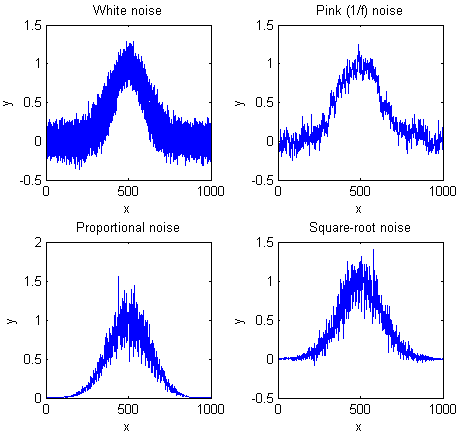
The Matlab/Octave function noisetest.m demonstrates
the
appearance and effect of different noise types. It
plots Gaussian peaks with four different types of
added noise: constant white noise, constant pink (1/f) noise,
proportional white noise, and square-root white noise, then fits
a Gaussian to each noisy data set and computes the average and
the standard deviation of the peak height, position, width and
area for each noise type. Type "help noisetest" at the command
prompt. The Matlab/Octave script SubtractTwoMeasurements.m
demonstrates the technique of subtracting two separate
measurements of a waveform to extract the random noise (but
it works only if the signal is stable, except for the
noise). Graphic.
Live
scripts
Both Matlab and Python have interactive
alternatives to conventional scripts. Live
Scripts in Matlab are interactive documents that
combine code, output, and formatted text in a single
environment called the Live Editor. (Live Scripts were
available starting in MATLAB R2016b). Python has Jupyter
Notebooks which are used to create an interactive
narrative around your code. Both make it easy to create
sharable interactive document with graphical user interface
devices such as pull-down menus, buttons, and sliders to
adjust numerical values interactively.
This
example shows four types of interactive controllers. Line 1
shows a button that opens a file browser that allow
you to navigate to a specific file, in this case a data file
that you want to process. Lines 4 and 5 show check boxes,
which are used to enable or disable optional sections of code.
Several lines show numeric sliders, which are used to
control continuous variables. Line 20 shows a drop-down
menu that allows multiple choices.
Live Scripts produce graphic
output in small windows on the right side of the Live editor
window, where you can copy, pan and zoom and export to png
files as usual using the mouse. You can also convert any Live
Script graphic into a standard figure window by clicking its
upper right corner; the standard figure window can then be
exported to other graphic formats, expanded to full screen,
printed, etc.
Live scripts are surprisingly easy to create by modifying a
conventional script. In Matlab, you can simply open a
conventional (.m) script in the Live Editor and insert the interface devices directly
into the script where the
numbers in assignment statements would have gone. When you
save it, it becomes a .mlx file. See AppendixAF.html for more detailed
instructions.
iSignal
iSignal is one of a group of
multi-purpose keystroke-operated Matlab functions that I have
developed that combine many of the techniques covered here; iSignal
can plot signals with pan and zoom controls, measure signal
and noise amplitudes in selected regions of the signal and compute
the S/N ratio of peaks. It is operated by simple key presses (e.g.
press K to display a list of keypress commands). Other
capabilities of iSignal include smoothing, differentiation, peak
sharpening and de-tailing, deconvolution, least-squares peak
measurement, etc.
Others in this group of interactive functions include iPeak,
which focuses on peak detection, iFilter,
which focuses on Fourier filtering, and ipf.m,
which focuses on iterative curve fitting. These functions
are ideal for initial explorations of complex signal because
they make it easy to select operations and adjust the
controls by simple key presses. These work even if you run
Matlab Online in a web browser, but they do not work on
Matlab Mobile. Note that the Octave versions,
ipfoctave.m, ipeakoctave.m, isignaloctave.m, and
ifilteroctave.m, use the < and > keys (with and
without shift) for pan and zoom.
For signals that contain
repetitive waveform patterns occurring in one continuous signal,
with nominally the same shape except for noise, the interactive
peak detector function iPeak has an ensemble
averaging function (Shift-E) can compute the
average of all the repeating waveforms. It works by detecting a
single reference peak in each repeat waveform in order to
synchronize the repeats (and therefore does not require that the
repeats be equally spaced or synchronized to an external
reference signal). To use this function, first adjust the peak
detection controls to detect only one peak in each repeat
pattern, then zoom in to isolate any one of those repeat
patterns, and then press Shift-E. The average waveform
is displayed in Figure 2 and saved as EnsembleAverage.mat" in
the current directory. See iPeakEnsembleAverageDemo.m
for a demonstration.


 usually
defined as the concentration that produces the smallest
detectable signal (Reference
90). A signal below the detection limit cannot be reliably
detected, that is, if the measurement is repeated, the signal
will often be "lost in the noise" and reported as zero. A signal
above the detection limit will be reliable detected and will
seldom or never reported as zero. The most common definition of
signal-to-noise ratio at the detection limit is 3. This is
illustrated in the figure on the left (created by the
Matlab/Octave script SNRdemo.m). This
shows a noisy signal in the form of a rectangular pulse. We
define the "signal" as the average signal magnitude during the
pulse, indicated by the red line, which is 3 ("signal" in line 3
of the script, which you can change). We define the "noise" as
the the standard deviation of the random noise on the baseline
before and after the pulse, which is about 1.0 (roughly 1/5 of
the peak-to-peak baseline noise indicated by the two black
horizontal lines). So the signal-to-noise ratio (SNR) in this
case is about 3, which is the most common definition of
detection limit. This means that this is the lowest signal that
can be reliably detected and that signals lower than this should
be reported as "undetectable".
usually
defined as the concentration that produces the smallest
detectable signal (Reference
90). A signal below the detection limit cannot be reliably
detected, that is, if the measurement is repeated, the signal
will often be "lost in the noise" and reported as zero. A signal
above the detection limit will be reliable detected and will
seldom or never reported as zero. The most common definition of
signal-to-noise ratio at the detection limit is 3. This is
illustrated in the figure on the left (created by the
Matlab/Octave script SNRdemo.m). This
shows a noisy signal in the form of a rectangular pulse. We
define the "signal" as the average signal magnitude during the
pulse, indicated by the red line, which is 3 ("signal" in line 3
of the script, which you can change). We define the "noise" as
the the standard deviation of the random noise on the baseline
before and after the pulse, which is about 1.0 (roughly 1/5 of
the peak-to-peak baseline noise indicated by the two black
horizontal lines). So the signal-to-noise ratio (SNR) in this
case is about 3, which is the most common definition of
detection limit. This means that this is the lowest signal that
can be reliably detected and that signals lower than this should
be reported as "undetectable". shows that all of the signal
points are above the highest baseline points. This graphic more
accurately represents what we judge when we look at a signal
like that in the previous graphic: a clear separation of signal
and baseline. The SNR of the peak has improved from 3.1 to 7.7
and the detection limit will be correspondingly reduced.
As a rule of thumb, the noise decreases by the roughly the
square root of the number of points averaged (sqrt(5)=2.2).
Higher values will further improve the SNR and reduce the
relative standard deviation of the average signal, but the
response time - which is the time it takes for the signal to
reach the average value - will become slower and slower as the
number of points averaged increases. This is shown by this graphic with 100 points
averaged. With a much lower signal, where the SNR is only 1.0,
the raw signal is barely detectable
visually, but with a 100 point average, the signal precision is good.
Digital averaging beats visual averaging in this case.
shows that all of the signal
points are above the highest baseline points. This graphic more
accurately represents what we judge when we look at a signal
like that in the previous graphic: a clear separation of signal
and baseline. The SNR of the peak has improved from 3.1 to 7.7
and the detection limit will be correspondingly reduced.
As a rule of thumb, the noise decreases by the roughly the
square root of the number of points averaged (sqrt(5)=2.2).
Higher values will further improve the SNR and reduce the
relative standard deviation of the average signal, but the
response time - which is the time it takes for the signal to
reach the average value - will become slower and slower as the
number of points averaged increases. This is shown by this graphic with 100 points
averaged. With a much lower signal, where the SNR is only 1.0,
the raw signal is barely detectable
visually, but with a 100 point average, the signal precision is good.
Digital averaging beats visual averaging in this case. 
 acoustical domain, white noise
sounds like a hiss. In measurement science, white noise
is fairly common, For example, quantization noise, Johnson-Nyquist
(thermal) noise, photon noise,
and the noise made by single-point
spikes all have white frequency distributions, and all have
in common their origin in discrete quantized instantaneous events,
such as the flow of individual electrons or photons.
acoustical domain, white noise
sounds like a hiss. In measurement science, white noise
is fairly common, For example, quantization noise, Johnson-Nyquist
(thermal) noise, photon noise,
and the noise made by single-point
spikes all have white frequency distributions, and all have
in common their origin in discrete quantized instantaneous events,
such as the flow of individual electrons or photons.  One way to observe this is to select a
segment of signal over which the signal amplitude varies widely,
fit the signal to a polynomial or
multiple peak model, and observe
how the residuals vary with signal amplitude. The graphic on the
left shows a real experimental signal, showing that the residuals
from a curve-fitting operation reveals that the noise increases
with signal amplitude. Another
example shows an example where the noise is almost
independent of the signal amplitude.
One way to observe this is to select a
segment of signal over which the signal amplitude varies widely,
fit the signal to a polynomial or
multiple peak model, and observe
how the residuals vary with signal amplitude. The graphic on the
left shows a real experimental signal, showing that the residuals
from a curve-fitting operation reveals that the noise increases
with signal amplitude. Another
example shows an example where the noise is almost
independent of the signal amplitude.  This is easily demonstrated by
a little simulation. In the example on the left, we start
with a set of 100,000 uniformly
distributed random numbers that have an equal chance of
having any value between certain limits - between 0 and +1
in this case (like the "rand" function in most spreadsheets
and Matlab/Octave). The graph in the upper left of the
figure shows the probability distribution, called a "histogram", of that random variable. Next,
we combine two sets of such independent,
uniformly-distributed random variables (changing the signs
so that the average remains centered at zero). The result
(shown in the graph in the upper right in the figure) has a
triangular distribution between -1 and +1, with the
highest point at zero, because there are many ways for the
difference between two random numbers to be small, but only
one way for the difference to be 1 or to -1 (that happens
only if one number is exactly zero and the other
is exactly 1). Next, we combine four independent
random variables (lower left); the resulting distribution
has a total range of -2 to +2, but it is even less likely
that the result be near 2 or -2 and many more ways
for the result to be small, so the distribution is narrower
and more rounded, and is already starting to be visually
close to a normal Gaussian distribution (shown for reference
in the lower right). If we combine more and more independent
uniform random variables, the combined probability
distribution becomes closer and closer to Gaussian (shown in
the bottom right). The Gaussian
distribution that we observe here is not forced by
prior assumption; rather, it arises naturally.
You
can download a Matlab script for this simulation from http://terpconnect.umd.edu/~toh/spectrum/CentralLimitDemo.m.
This is easily demonstrated by
a little simulation. In the example on the left, we start
with a set of 100,000 uniformly
distributed random numbers that have an equal chance of
having any value between certain limits - between 0 and +1
in this case (like the "rand" function in most spreadsheets
and Matlab/Octave). The graph in the upper left of the
figure shows the probability distribution, called a "histogram", of that random variable. Next,
we combine two sets of such independent,
uniformly-distributed random variables (changing the signs
so that the average remains centered at zero). The result
(shown in the graph in the upper right in the figure) has a
triangular distribution between -1 and +1, with the
highest point at zero, because there are many ways for the
difference between two random numbers to be small, but only
one way for the difference to be 1 or to -1 (that happens
only if one number is exactly zero and the other
is exactly 1). Next, we combine four independent
random variables (lower left); the resulting distribution
has a total range of -2 to +2, but it is even less likely
that the result be near 2 or -2 and many more ways
for the result to be small, so the distribution is narrower
and more rounded, and is already starting to be visually
close to a normal Gaussian distribution (shown for reference
in the lower right). If we combine more and more independent
uniform random variables, the combined probability
distribution becomes closer and closer to Gaussian (shown in
the bottom right). The Gaussian
distribution that we observe here is not forced by
prior assumption; rather, it arises naturally.
You
can download a Matlab script for this simulation from http://terpconnect.umd.edu/~toh/spectrum/CentralLimitDemo.m.


