Fourier filter

[Simple Example]   [Command line function]   [Segmented Fourier filter]   [Interactive Fourier Filter]   [Live Script Fourier filter]   [Application of a narrow bandpass filter]   [Live Script Fourier Filter]

The Fourier filter is a type of filtering function that is based on manipulation of specific frequency components of a signal. It works by taking the Fourier transform of the signal, then attenuating or amplifying specific frequencies, and finally inverse transforming the result. In many science measurements, such as spectroscopy and chromatography, the signals are relatively smooth shapes that can be represented by a surprisingly small number of Fourier components. For example, the animation below (script) shows in the top panel a signal of three smooth peaks, with peak heights of 1, 2, and 3, where the x-axis is time in seconds. The middle panel shown the first 51 frequencies of its Fourier spectrum (zero through 50). In this case the x-axis is both the frequency in Hz and the Fourier component number (because the duration of the signal is exactly 1 second). The amplitude of the Fourier components is strongest at low frequencies and drops to near zero at 25 Hz.

z

The bottom panel shows in this figure the signal re-constructed by inverse transforming the first "n" Fourier components. The animation (visible in a web browser) shows the result of using the frequencies between 1 through 25 progressively. The reconstructed signal starts as a single sine wave and becomes progressively more complex as more frequencies are added, until it is visually indistinguishable from the original signal when 25 frequencies are included. But notice what the reconstructed signal looks like when it gets to 16 frequencies; the amplitude has already dropped very low and there is relatively little amplitude in the remaining frequencies. The three peaks are rendered well but the baseline has a distinct ripple. That is caused by the abrupt cut-off of the frequencies beyond that point, which can be avoided by using a filter with an adjustable filter shape that allows the cut-off rate to be controlled.

The figure below shows the same three-peak signal, but with the addition of random white noise with a standard deviation equal to the the peak height of the smallest peak (line 14 of the same script). White noise has equal amplitude at all frequencies, whereas most of the peak signal is concentrated in the first 25 frequencies, so we can expect that most but not all of the noise can be eliminated by employing a low-pass filter with a cut-off frequency around 25 Hz. The result (bottom panel) shows the three peaks with their position and peak heights approximately intact. Obviously the noise below 25 Hz remains, which is why the signal is imperfect.

The optimization of the Fourier filter for the signal-to-noise (SNR) ratio of peak signals faces the same compromise as conventional smoothing functions; namely, the optimum SNR is achieved when the peak height is less than the noiseless maximum. For example, the script GaussianSNRFrequencyReconstruction.m shows that the optimum SNR is reached when the peak height is about half the true value, but the peak area is the same.

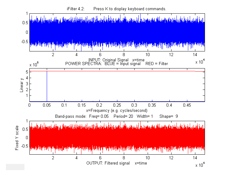
Adjustable filter shape. A more dramatic example is shown the figure below. In this case, the signal (top left) seems to be only random high-frequency noise, and its Fourier spectrum (top right) shows that high-frequency components dominate the spectrum over much of its frequency range (script). In the bottom left figure, the Fourier spectrum is expanded in the X and Y directions to show the low-frequency region more clearly  There, the series of relatively smooth bumps with peaks at the 1st, 20th, and 40th frequencies, are most likely the actual signal. Working on the hypothesis that the components above the 40th harmonic are increasingly dominated by noise, a more versatile  Fourier filter function (FouFilter.m) can be used to gradually reduce the higher harmonics and to reconstruct the signal from the modified Fourier transform (red line). The result after inverse Fourier transforming (bottom right) shows the signal actually contains two partly overlapping Lorentzian peaks that were totally obscured by noise in the original signal.

 

ffty=fft(y); % ffty is the fft of y
lfft=length(ffty); % Length of the FFT
% All frequencies between n and lfft-n in the fft
% are set to zero.
ffty(n:lfft-n)=0;
fy=real(ifft(ffty)); % Real part of the inverse fft

Here, n is the number of frequencies that are passed; all others are simply eliminated. The function form of this operation is flp.m. This is the minimal essence of a Fourier filter. The script flptest.m demonstrates its use (figure on the right). The is not really a practical filter, however, because its abrupt cutoff usually results in ringing on the baseline, as shown above.

General-purpose Fourier filter function. To make the Fourier filter more generally useful, we should add code to include not only low-pass, but also high-pass, band pass, and band reject filter modes, plus a provision for more gentle and variable cut-off rates. This, and more, is done in the following section. The custom Matlab/Octave function FouFilter.m can serve as a bandpass or bandreject (notch) filter with variable cut-off rate. (Version 2, March, 2019, correction thanks to Dr. Raphael Attie, NASA/Goddard Space Flight Center). It has the form [ry,fy,ffilter,ffy] = FouFilter(y, samplingtime, centerfrequency, frequencywidth, shape, mode), where y is the time-series signal vector, 'samplingtime' is the total duration of sampled signal in sec, millisec, or microsec; 'centerfrequency' and 'frequencywidth' are the center frequency and width of the filter in Hz, KHz, or MHz, respectively; 'Shape' determines the sharpness of the cut-off. If shape = 1, the filter is Gaussian; as shape increases the filter shape becomes more and more rectangular. Set mode = 0 for band-pass filter, mode = 1 for band-reject (notch) filter. Set centerfrequency to zero for a low-pass filter. FouFilter returns the filtered signal in 'ry'. It can handle signals of virtually any length, limited only by the memory in your computer. Here are two examples of its application: TestFouFilter.m demonstrates a Fourier bandpass filter applied to a noisy 100 Hz sine wave which appears in the middle third of the signal record. TestFouFilter2.m is an animated demonstration of the Fourier bandpass filter applied to a noisy 100 Hz sine wave signal, with the filter center frequency swept from 50 to 150 Hz. Both requires the FouFilter.m function in the Matlab/Octave path.

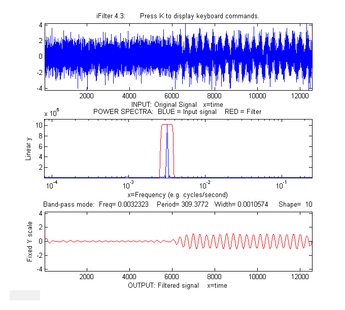
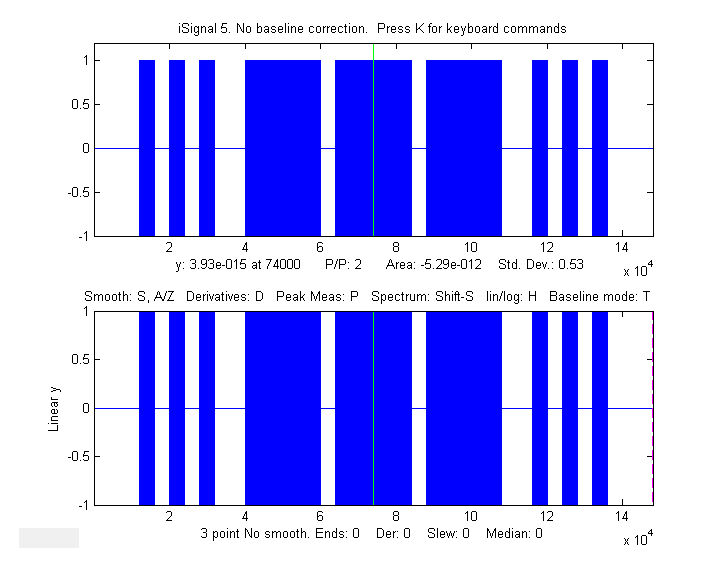
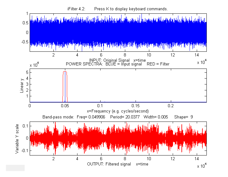
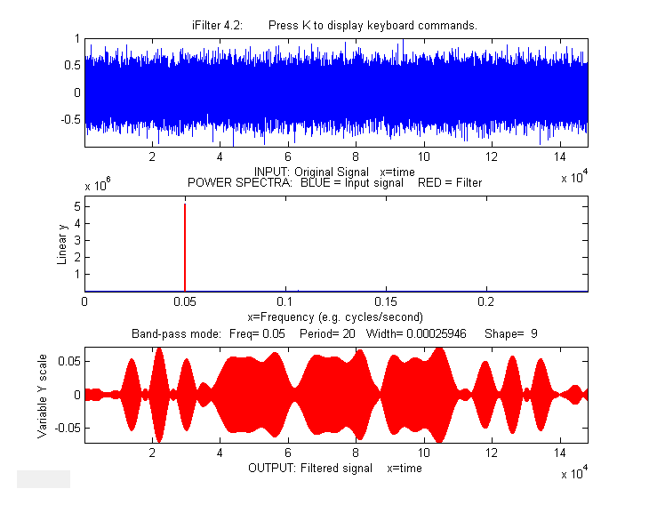
MorseCode.m is a script that uses iFilter to demonstrate the abilities and limitations of Fourier filtering. It creates a pulsed fixed 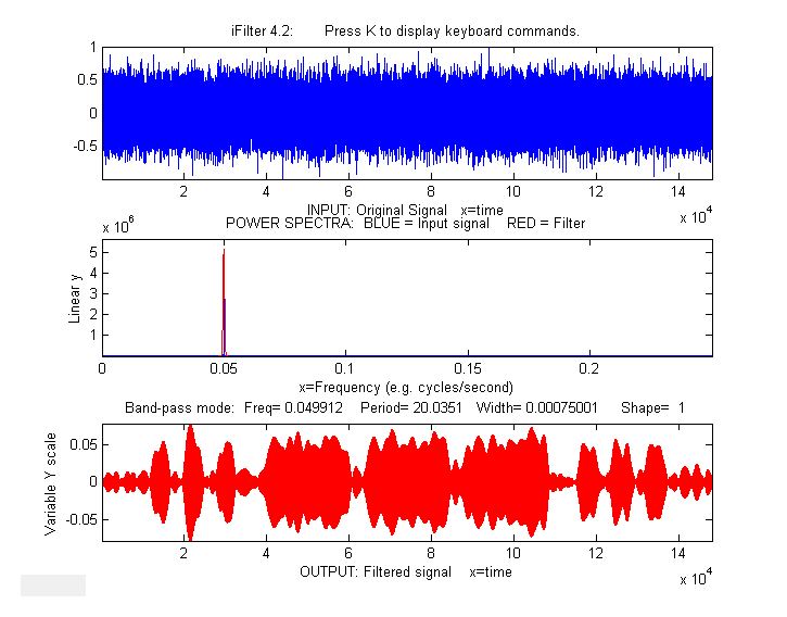frequency (0.05) sine wave that spells out "SOS" in Morse code (dit-dit-dit/dah-dah-dah/dit-dit-dit), adds random white noise so that the SNR is extremely poor (about 0.1 in this example). 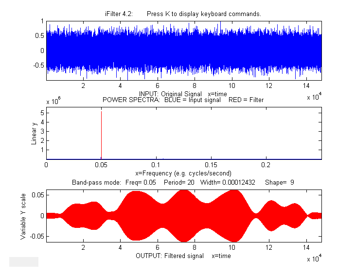The white noise has a frequency spectrum that is spread out over the entire range of frequencies; the signal itself is concentrated mostly at a fixed frequency (0.05) but the presence of the Morse Code pulses spreads out its spectrum over a narrow frequency range of about 0.0004. This suggests that a Fourier bandpass filter tuned to the signal frequency might be able to isolate the signal from the noise. As the bandwidth is reduced, the signal-to-noise ratio improves and the signal begins to emerges from the noise until it becomes clear, but if the bandwidth is too narrow, the step response time is too slow to give distinct "dits" and "dahs". The step response time is inversely proportional to the bandwidth. (Use the ? and " keys to adjust the bandwidth. Press 'P' or the Spacebar to hear the sound). 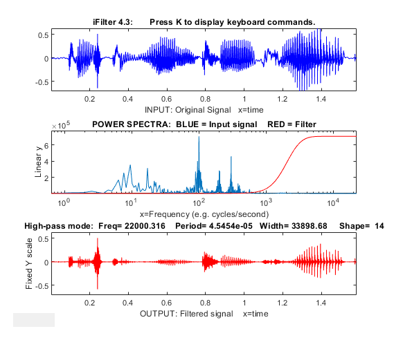You can actually hear that sine wave component better than you can see it in the waveform plot (upper panel), because the ear works like a spectrum analyzer, with separate nerve endings assigned to to specific frequencies, whereas the eye analyzes the graph spatially, looking at the overall amplitude and not at individual frequencies. 

FourierFilterTool.mlx is a Live Script version of the interactive Fourier filter iFilter.m. It can perform six different types of Fourier filtering on your own data stored in .csv or .xls format. The graphic display (above right) is essentially identical to the iFilter.m function.

Note: To view the figures to the right of the control panel as shown above, right-click on the right-hand panel and select "Disable synchronous scrolling".

Clicking the "Open data file" button in line 1 opens a file browser, allowing you to navigate to your data file (in .csv or .xlsx format; the script assumes that your x,y data are in the first two columns; you can change that in lines 27 and 28). In the case shown here, the data file is 'ThreeSines.csv', shown as the 'file' variable in the Matlab workspace. The startpc and endpc sliders in lines 5 and 7 allow you to select which portion of the data range to process, from 0% to 100% of the total range of the data file.

There are drop-down menus and sliders to select the type of filter type, center frequency, filter width, filter shape, linear or log axes, time or frequency mode, and fixed or variable Y axis for the output.

Clicking the checkbox labeled "PlayOutputAsSound" will send the output waveform to the system's speaker each time any control is changed. Un-check that box to cancel.