Differentiation

[Basic Properties of Derivatives]   [Applications of Differentiation]   [Peak detection]   [Derivative Spectroscopy]   [Trace Analysis]   [The Importance of Smoothing Derivatives]   [Video Demonstrations]   [Spreadsheets]  [Differentiation in Matlab and Octave]   [Live script]   [Other Interactive tools]  [Have a question? Email me]

where X'_j and Y'_j are the X and Y values of the j^th point of the derivative, n = number of points in the signal, and X is the difference between the X values of adjacent data points. A commonly used variation of this algorithm computes the average slope between three adjacent points:

This is called a central-difference method; its advantage is that it does not involve a shift in the x-axis position of the derivative. It's also possible to compute gap-segment derivatives in which the x-axis interval between the points in the above expressions is greater than one; for example, Y_j-2 and Y_j+2, or  Y_j-3 and Y_j+3, etc. It turns out that this is equivalent to applying a moving-average (rectangular) smooth in addition to the derivative. 

The second derivative is the derivative of the derivative: it is a measure of the curvature of the signal, that is, the rate of change of the slope of the signal. It can be calculated by applying the first derivative calculation twice in succession. The simplest algorithm for direct computation of the second derivative in one step is

Similarly, higher derivative orders can be computed using the appropriate sequence of coefficients: for example +1, -2, +2, -1 for the third derivative and +1, -4, +6, -4, +1 for the 4^th  derivative, although these derivatives can also be computed simply by taking successive lower order derivatives. The first derivative can be interpreted as the slope of the original at each point, and the second derivative as the curvature, but beyond that we have no single-word labels; each derivative is just the rate of change of the one before it.

The Savitzky-Golay smooth can also be used as a differentiation algorithm with the appropriate choice of input arguments; it combines differentiation and smoothing into one algorithm.

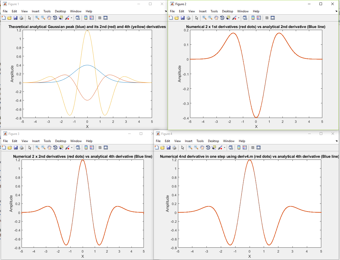
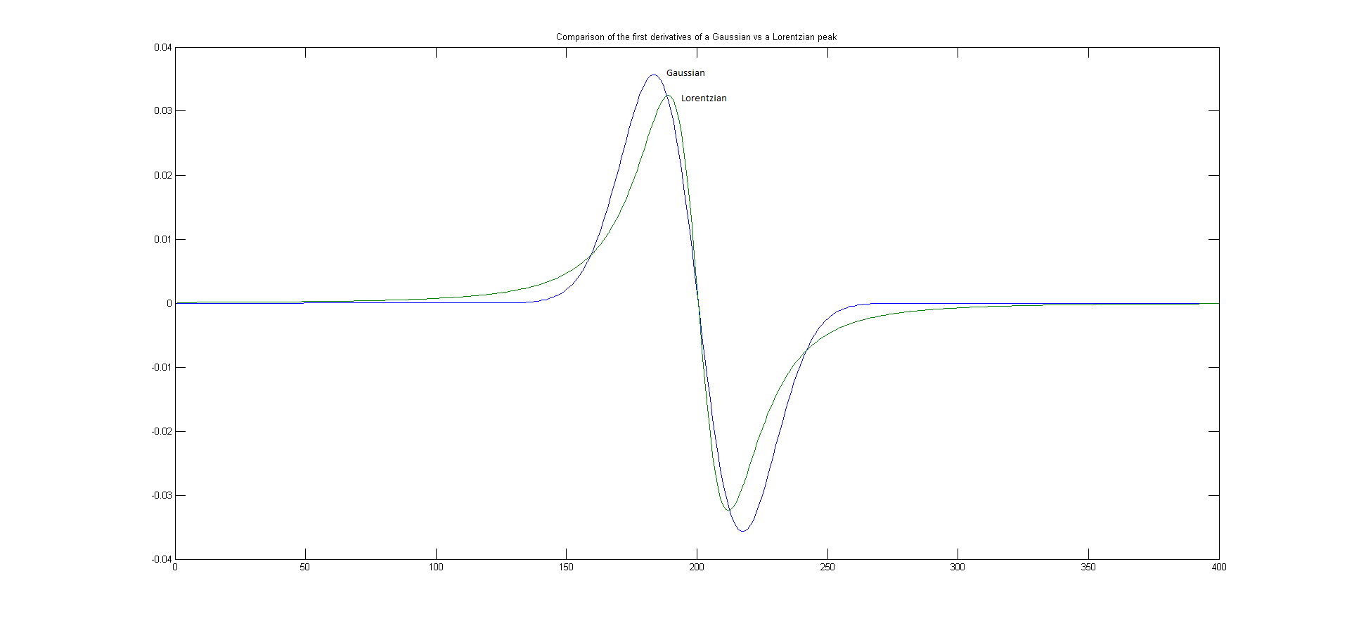
The accuracy of numerical differentiation is demonstrated by the Matlab/Octave script GaussianDerivatives.m (graphic), which compares the exact analytical expressions for the derivatives of a Gaussian (readily obtained from Wolfram Alpha) to the numerical values obtained by the expressions above, demonstrating that the shape and amplitude of the derivatives are an exact match as long as the sampling interval is not too coarse. It also demonstrates that the numerical nth derivative can be obtained exactly by applying n successive first differentiations.  Ultimately, the numerical precision limitation of the computer can be a limitation in some extreme cases.

Basic Properties of Derivative Signals

The figure on the left shows the results of the successive differentiation of a computer-generated Gaussian peak signal (click to see the full-sized figure). The signal in each of the four windows is the first derivative of the one before it; that is, Window 2 is the first derivative of Window 1, Window 3 is the first derivative of Window 2, Window 3 is the second derivative of Window 1, and so on. You can predict the shape of each signal by recalling that the derivative is simply the slope of the original signal: where a signal slopes up, its derivative is positive; where a signal slopes down, its derivative is negative; and where a signal has zero slope, its derivative is zero. (Matlab/Octave code for this figure.)

The sigmoidal signal shown in Window 1 has an inflection point (point where where the slope is maximum) at the center of the x axis range. This corresponds to the maximum in its first derivative (Window 2) and to the zero-crossing (point where the signal crosses the x-axis going either from positive to negative or vice versa) in the second derivative in Window 3. This behavior can be useful for precisely locating the inflection point in a sigmoid signal, by computing the location of the zero-crossing in its second derivative. 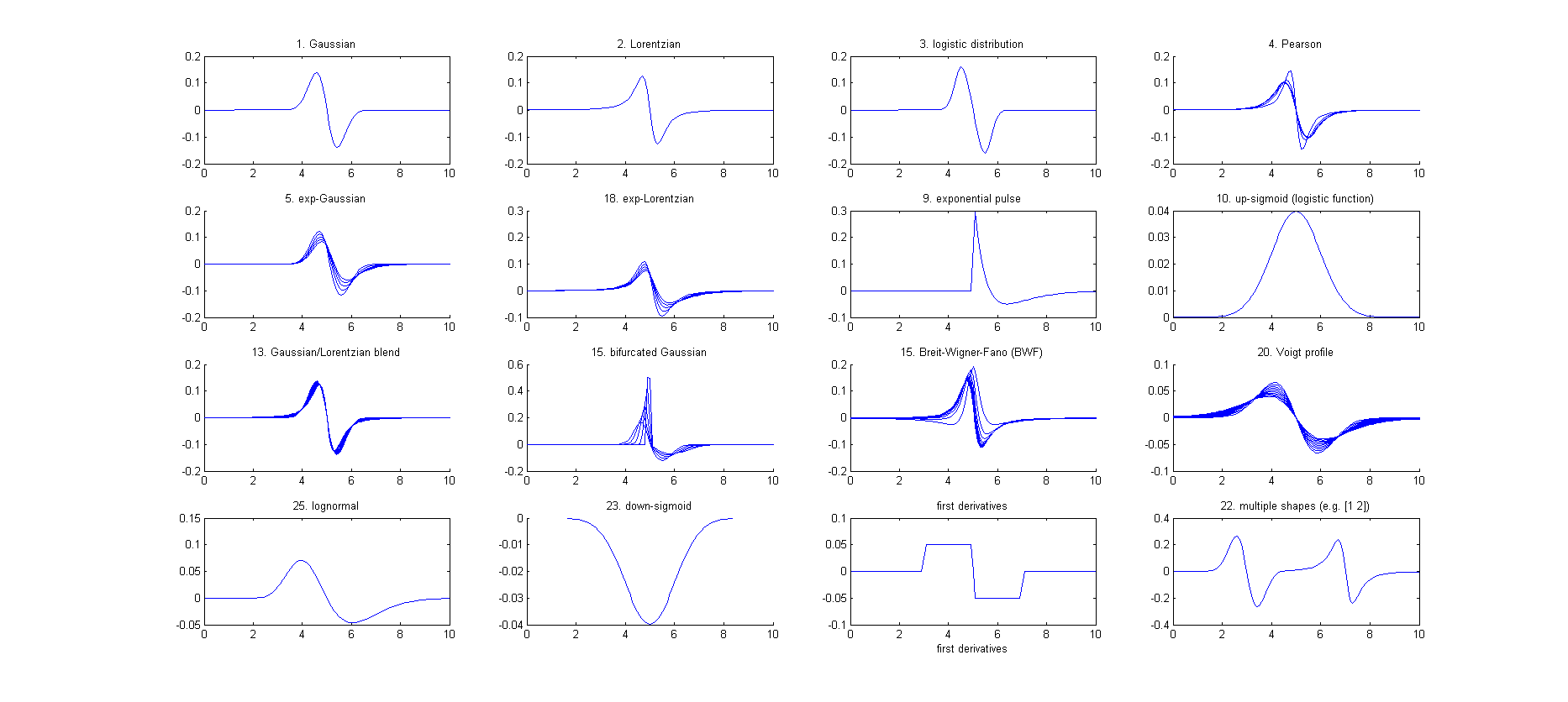Similarly, the location of the maximum in a peak-type signal can be computed precisely by computing the location of the zero-crossing in its first derivative. 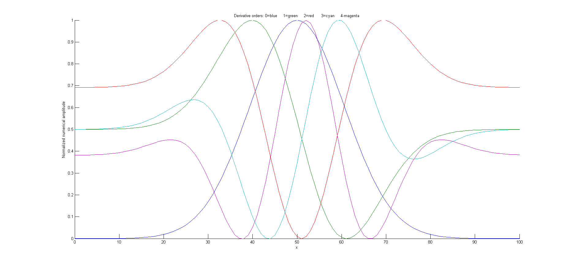Different peak shapes have different derivatives shapes: the Matlab/Octave function DerivativeShapeDemo.m demonstrates the first derivative forms of 16 different model peak shapes (graphic). Any smooth peak shape with a single maximum has sequential derivatives that exhibit a series of alternating maxima and minima, the total number of which is one more than the derivative order. The even-order derivatives have a maximum or a minimum at the peak center, and the odd-order derivatives have a zero-crossing at the peak center (Graphic, Matlab/Octave code). You can also see here that the numerical magnitude of the derivatives (y-axis values) is much less than the original signal, because derivatives are the differences between adjacent y values, divided by the independent variable increment. (It's the same reason the odometer in your car usually displays a much larger number than the speedometer; the speedometer is essentially the first derivative of the odometer).

An important property of the differentiation of peak-type signals is the effect of the peak width on the amplitude of derivatives. The figure on the left shows the results of the successive differentiation of two computer-generated Gaussian bands (click to see the full-sized figure). The two bands have the same amplitude (peak height) but one of them is exactly twice the width of the other. As you can see, the wider peak has the smaller derivative amplitude, and the effect becomes more noticeable at higher derivative orders. In general, it is found that that the amplitude of the n^th derivative of a peak is inversely proportional to the n^th power of its width, for signals having the same shape and amplitude. Thus differentiation in effect discriminates against wider peaks and the higher the order of differentiation the greater the discrimination. This behavior can be useful in quantitative analytical applications for detecting peaks that are superimposed on and obscured by stronger but broader background peaks. (Matlab/Octave code for this figure). The amplitude of a derivative of a peak also depends on the shape of the peak and is directly proportional to its peak height. Gaussian and Lorentzian peak shapes have slightly different first and second derivative shapes and amplitudes. The amplitude of the n^th derivative of a Gaussian peak of height H and width W can be estimated by the empirical equation H*(10^(0.027*n^2+n*0.45-0.31)).*W^(-n), where W is the full width at half maximum (FWHM) measured in the number of x,y data points.

Although differentiation changes the shape of peak-type signals drastically, a periodic signal like a sine wave signal behaves very differently. The derivative of a sine wave of frequency f is a phase-shifted sine wave, or cosine wave, of the same frequency and with an amplitude that is proportional to f, as can be demonstrated in Wolfram Alpha. The derivative of a periodic signal containing several sine components of different frequency will still contain those same frequencies, but with altered amplitudes and phases. For this reason, when a music or speech signal is differentiated, the music or speech is still completely recognizable, but with the high frequencies increased in amplitude compared to the low frequencies, and as a result, it sounds "thin" or "tinny". See this demonstration for an example.

Applications of Differentiation

A simple example of the application of differentiation of experimental signals is shown in the figure below. This signal is typical of the type of signal recorded in amperometric titrations and some kinds of thermal analysis and kinetic experiments: a series of straight line segments of different slope. The objective is to determine how many segments there are, where the breaks between then fall, and the slopes of each segment. This is difficult to do from the raw data, because the slope differences are small and the resolution of the computer screen display is limiting. The task is much simpler if the first derivative (slope) of the signal is calculated (below right). Each segment is now clearly seen as a separate step whose height (y-axis value) is the slope. The y-axis now takes on the units of dy/dx. Note that in this example the steps in the derivative signal are not completely flat, indicating that the line segments in the original signal were not perfectly straight. This is most likely due to random noise in the original signal. Although this noise was not particularly evident in the original signal, it is more noticeable in the derivative.

The signal on the left seems to be a more-or-less straight line, but its numerically calculated derivative (dx/dy), plotted on the right, shows that the line actually has several approximately straight-line segments with distinctly different slopes and with well-defined breaks between each segment.

It is commonly observed that differentiation degrades signal-to-noise ratio, unless the differentiation algorithm includes smoothing that is carefully optimized for each application. Numerical algorithms for differentiation are as numerous as for smoothing and must be carefully chosen to control signal-to-noise degradation.

A classic use of second differentiation in chemical analysis is in the location of endpoints in potentiometric titration. In most titrations, the titration curve has a sigmoidal shape and the endpoint is indicated by the inflection point, the point where the slope is maximum and the curvature is zero. The first derivative of the titration curve will therefore exhibit a maximum at the inflection point, and the second derivative will exhibit a zero-crossing at that point. Maxima and zero crossings are usually much easier to locate precisely than inflection points.

The figure above shows a pH titration curve of a very weak acid with a strong base, with volume in mL on the X-axis and pH on the Y-axis. The volumetric equivalence point (the "theoretical" endpoint) is 20 mL. The endpoint is the point of greatest slope; this is also an inflection point, where the curvature of the signal is zero. With a weak acid such as this, it is difficult to locate this point precisely from the original titration curve. The second derivative of the curve is shown in Window 2 on the right. The zero crossing of the second derivative corresponds to the endpoint and is much more precisely measurable. Note that in the second derivative plot, both the x-axis and the y-axis scales have been expanded to show the zero crossing point more clearly. The dotted lines show that the zero crossing falls at about 19.4 mL, close to the theoretical value of 20 mL.

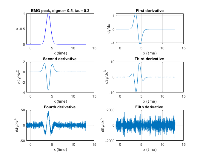
Derivatives can also be used as a simple way to detect unexpected asymmetry in otherwise symmetrical peaks. For example, a pure Gaussian peaks is symmetrical but, if subjected to exponential broadening, can become asymmetrical. If the degree of broadening is small, it can be difficult to detect visually; that is where differentiation can help. DerivativeEMGDemo.m (graphic) shows the 1st through 5th derivatives of a slightly exponentially broadened Gaussian (EMG); of those derivatives, the second clearly shows unequal positive peaks that would be expected to be equal for a purely symmetrical peak. The higher derivatives offer no clear advantage and are more susceptible to white noise in the signal. 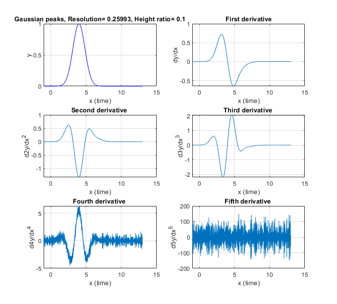For another example, if a Gaussian peak is heavily overlapped by a smaller peak, the result is usually asymmetrical. The script DerivativePeakOverlapDemo (graphic) shows the 1st through 5th derivatives of two overlapping Gaussians where the second peak is so small and so close that it's impossible to discern visually, but again the second derivative shows the asymmetry clearly by comparing the heights of the two positive peaks. DerivativePeakOverlap.m detects the minimum extent of peak overlap by the first and second derivatives, looking for the point at which two peaks are visible; for each trial separation, it prints out the separation, resolution, and the number of peaks detected in the first and second derivatives.

Peak detection

 Another common use of differentiation is in the detection of peaks in a signal. It's clear from the basic properties described in the previous section that the first derivative of a peak has a downward-going zero-crossing at the peak maximum, which can be used to locate the x-value of the peak, as shown on the right (script). If there is no noise in the signal, then any data point that has lower values on both sides of it will be a peak maximum. But there is always at least a little noise in real experimental signals, and that will cause many false zero-crossings simply due to the noise. To avoid this problem, one popular technique smooths the first derivative of the signal first, before looking for downward-going zero-crossings, and then takes only those zero crossings whose slope exceeds a certain predetermined minimum (called the "slope threshold") at a point where the original signal amplitude exceeds a certain minimum (called the "amplitude threshold"). By carefully adjusting the smooth width, slope threshold, and amplitude threshold, it is possible to detect only the desired peaks over a wide range of peak widths and ignore peaks that are too small, too wide, or too narrow. Moreover, because smoothing can distort peak signals, reducing peak heights, and increasing peak widths, this technique can be extended to measure the position, height, and width of each peak by least-squares curve-fitting of a segment of original unsmoothed signal near the top of the peak (where the signal-to-noise ratio is usually the best). Thus, even if heavy smoothing is necessary to provide reliable discrimination against noise peaks, the peak parameters extracted by curve fitting are not distorted and the effect of random noise in the signal is reduced by curve fitting over multiple data points in the peak. This technique has been implemented in Matlab/Octave and in spreadsheets.

Peak detection algorithms like this are widely applied in spectroscopy, biomedical research, environmental monitoring, financial analysis, image processing, neuroscience, physics and material science, chemistry and chromatography, speech and audio processing (reference 100).

Derivative Spectroscopy

In spectroscopy, the differentiation of spectra is a widely used technique, particularly in infra-red, u.v.-visible absorption, fluorescence, and reflectance spectrophotometry, referred to as derivative spectroscopy. Derivative methods have been used in analytical spectroscopy for three main purposes:

(a) spectral discrimination, as a qualitative fingerprinting technique to accentuate small structural differences between nearly identical spectra;
(b) spectral resolution enhancement, as a technique for increasing the apparent resolution of overlapping spectral bands in order to more easily determine the number of bands and their wavelengths;
(c) quantitative analysis, as a technique for the correction for irrelevant background absorption and as a way to facilitate multicomponent analysis.  (Because differentiation is a linear technique, the amplitude of a derivative is proportional to the amplitude of the original signal, which allows quantitative analysis applications employing any of the standard calibration techniques). Most commercial spectrophotometers now have built-in derivative capability. Some instruments are designed to measure the spectral derivatives optically, by means of dual wavelength or wavelength modulation designs.

Because of the fact that the amplitude of the n^th derivative of a peak-shaped signal is inversely proportional to the n^th power of the width of the peak, differentiation may be employed as a general way to discriminate against broad spectral features in favor of narrow components. This is the basis for the application of differentiation as a method of correction for background signals in quantitative spectrophotometric analysis. Very often in the practical applications of spectrophotometry to the analysis of complex samples, the spectral bands of the analyte (i.e. the compound to be measured) are superimposed on a broad, gradually curved background. Background of this type can be reduced by differentiation.

This is illustrated by the figure above, which shows a simulated UV spectrum (absorbance vs wavelength in nm), with the green curve representing the spectrum of the pure analyte and the red line representing the spectrum of a mixture containing the analyte plus other compounds that give rise to the large sloping background absorption. The first derivatives of these two signals are shown in the center; you can see that the difference between the pure analyte spectrum (green) and the mixture spectrum (red) is reduced. This effect is considerably enhanced in the second derivative, shown on the right. In this case the spectra of the pure analyte and of the mixture are almost identical. In order for this technique to work, it is necessary that the background absorption be broader (that is, have lower curvature) than the analyte spectral peak, but this turns out to be a rather common situation. Because of their greater discrimination against broad background, second (and sometimes even higher-order) derivatives are often used for such purposes. See DerivativeDemo.m for a Matlab/Octave demonstration of this application.

It is sometimes (mistakenly) said that differentiation "increases the sensitivity" of analysis. You can see how it would be tempting to say something like that by inspecting the three figures above; it does seems that the signal amplitude of the derivatives is greater than that of the original analyte signal (at least graphically). However, it is not valid to compare the amplitudes of signals and their derivatives because they have different units. The units of the original spectrum are absorbance; the units of the first derivative are absorbance per nm, and the units of the second derivative are absorbance per nm². You can't compare absorbance to absorbance per nm any more than you can compare miles to miles per hour. (It's meaningless, for instance, to say that a speed of 30 miles per hour is greater than a distance of 20 miles.) You can, however, compare the signal-to-background ratio and the signal-to-noise ratio. For instance, in the above example, it would be valid to say that the signal-to-background ratio is increased in the derivatives.

Loosely speaking, the opposite of differentiation is integration, so if you are given a first derivative of a signal, you might expect to regenerate the original (zeroth derivative) by integration. However, there is a catch; the constant term in original signal (like a flat baseline) is completely lost in differentiation; integration can not restore it. So strictly speaking, differentiation represents a net loss of information, and therefore differentiation is used only in situations where the constant term in the original signal is not of interest.

There are several ways to measure the amplitude of a derivative spectrum for quantitative analysis: the absolute value of the derivative at a specific wavelength, the value of a specific feature (such as a maximum), or the difference between a maximum and a minimum. Another widely-used technique is the zero-crossing measurement - taking readings derivative amplitude at the wavelength where an interfering peak crosses the zero on the y (amplitude) axis. In all these cases, it's important to measure the standards and the unknown samples in exactly the same way.  Also, because the amplitude of a derivative of a peak depends strongly on its width, it's important to control environmental factors that might change spectral peak width subtlety, such as temperature.

Trace Analysis

One of the widest uses of the derivative signal processing technique in practical analytical work is in the measurement of small amounts of substances in the presence of large amounts of potentially interfering materials. In such applications it is common that the analytical signals are weak, noisy, and superimposed on large background signals. Measurement precision is often degraded by sample-to-sample baseline shifts due to non-specific broadband interfering absorption, non-reproducible cuvette (sample cell) positioning, dirt or fingerprints on the cuvette walls, imperfect cuvette transmission matching, and solution turbidity. Baseline shifts from these sources are usually either wavelength-independent (light blockage caused by bubbles or large suspended particles) or exhibit a weak wavelength dependence (small-particle turbidity). Therefore it can be expected that differentiation will in general help to discriminate relevant absorption from these sources of baseline shift. An obvious benefit of the suppression of broad background by differentiation is that variations in the background amplitude from sample to sample are also reduced. This can result in improved precision or measurement in many instances, especially when the analyte signal is small compared to the background and if there is a lot of uncontrolled variability in the background. An example of the improved ability to detect trace component in the presence of strong background interference is shown in this figure:

The spectrum on the left shows a weak shoulder near the center due to a small concentration of the substance that is to be measured (e.g. the active ingredient in a pharmaceutical preparation). It is difficult to measure the intensity of this peak because it is obscured by the strong background caused by other substances in the sample. The fourth derivative of this spectrum is shown on the right. The background has been almost completely suppressed and the analyte peak now stands out clearly, facilitating measurement.

The spectrum on the left shows a weak shoulder near the center due to the analyte. The signal-to-noise ratio is very good in this spectrum, but in spite of that the broad, sloping background obscures the peak and makes quantitative measurement very difficult. The fourth derivative of this spectrum is shown on the right. The background has been almost completely suppressed and the analyte peak now stands out clearly, facilitating measurement. An even more dramatic case is shown below. This is essentially the same spectrum as in the figure above, except that the concentration of the analyte is ten times lower. The question is: is there a detectable amount of analyte in this spectrum? This is quite impossible to say from the normal spectrum, but inspection of the fourth derivative (right) shows that the answer is yes. Some noise is clearly evident here, but nevertheless the signal-to-noise ratio is sufficiently good for a reasonable quantitative measurement.

This use of signal differentiation has become widely used in quantitative spectroscopy, particularly for quality control in the pharmaceutical industry. In that application the analyte would typically be the active ingredient in a pharmaceutical preparation and the background interferences might arise from the presence of fillers, emulsifiers, flavoring or coloring agents, buffers, stabilizers, or other excipients.  Of course, in trace analysis applications, care must be taken to optimize signal-to-noise ratio of the instrument as much as possible.

Although it will eventually be shown that more advanced techniques such as curve fitting can also perform many of these quantitative measurement tasks quite well, the derivative techniques have the advantage of conceptual and mathematical simplicity and an easily-understood graphical way of presenting presenting data.

Derivatives and Noise: The Importance of Smoothing

It is often said that "differentiation increases the noise". That is true, but it is not the main problem. In fact, computing the unsmoothed first derivative of a set of random numbers increases its standard deviation by only the square root of 2, simply due to the usual propagation of errors of the sum or difference between two numbers. As an example, the standard deviation (std) of the numbers generated by the Matlab/Octave randn() function is 1.0 and its first derivative std(deriv1(randn(size(1:10000)))) equals about 1.4. But even a little bit of smoothing applied to the derivative will reduce this standard deviation greatly, e.g. std(fastsmooth(deriv1(randn(size(1:10000))),2,3)) equals about 0.4. More important is the fact that the signal-to-noise ratio of an unsmoothed derivative is almost always much lower (poorer) than that of the original signal, mainly because the numerical amplitude of the derivative is usually much smaller (as you can see for yourself in all the examples on this page). But smoothing is always used in any practical application to control this problem; with optimal smoothing, the signal-to-noise of a derivative can actually be greater than the unsmoothed original. For the successful application of differentiation in quantitative analytical applications, it is essential to use differentiation in combination with sufficient smoothing, in order to optimize the signal-to-noise ratio. This is illustrated in the figure on the left. (Matlab/Octave code for this figure.) Window 1 shows a Gaussian band with a small amount of added white noise. Windows 2, 3, and 4, show the first derivative of that signal with increasing smooth widths. As you can see, without sufficient smoothing, the signal-to-noise ratio of the derivative can be substantially poorer than the original signal. However, with adequate amounts of smoothing, the signal-to-noise ratio of the smoothed derivative can be better than that of the unsmoothed original. This effect is even more striking in the second derivative, as shown on the right (Matlab/Octave code for this figure). In this case, the signal-to-noise ratio of the unsmoothed second derivative (Window 2) is so poor you can not even see the signal visually, but the smoothed second derivative looks fine. Differentiation does not actually add noise to the signal; if there were no noise at all in the original signal, then the derivatives would also have no noise (exception: see Appendix V).

What is particularly interesting about the noise in these derivative signals, however, is their "color". This noise is not white; rather, it is blue - that is, it has much more power at high frequencies than white noise. The consequence of this is that the noise in differentiated signal is easily reduced greatly by smoothing, as demonstrated above.

It makes no difference whether the smooth operation is applied before or after the differentiation. What is important, however, is the nature of the smooth, its smooth ratio (ratio of the smooth width to the width of the original peak), and the number of times the signal is smoothed. The optimum values of smooth ratio for derivative signals is approximately 0.5 to 1.0. For a first derivative, two applications of a simple rectangular smooth (or one application of a triangular smooth) is adequate. For a second derivative, three applications of a simple rectangular smooth or two applications of a triangular smooth is adequate. The general rule is: for the n^th derivative, use at least n+1 applications of a rectangular smooth. (The Matlab signal processing program iSignal automatically provides the desired type of smooth for each derivative order).

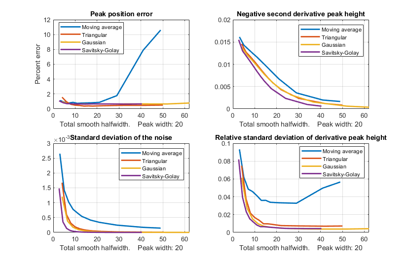
A quantitative comparison of smoothing the derivatives is performed by the script MultiPeakDerivativeOptimization.m, which analyzes the second derivatives of Gaussian peaks smoothed by moving average, triangular, Gaussian, and Suavity-Golay smooth types(graphic).

If the peak widths vary substantially across the signal recording - for example, if the peaks get regularly wider as the x-value increases - then it may be helpful to use an adaptive segmented smooth, which makes the smooth width vary across the signal.

Smoothing derivative signals usually results in a substantial attenuation of the derivative amplitude; in the figure on the right above, the amplitude of the most heavily smoothed derivative (in Window 4) is much less than its less-smoothed version (Window 3). However, this won't be a problem in quantitative analysis applications, as long as the standard (analytical) curve is prepared using the exact same derivative, smoothing, and measurement procedure as is applied to the unknown samples. Because differentiation and smoothing are both linear techniques, the amplitude of a smoothed derivative is exactly proportional to the amplitude of the original signal, which allows quantitative analysis applications employing any of the standard calibration techniques. As long as you apply the same signal-processing techniques to the standards as well as to the samples, everything works.

Because of the different kinds and degrees of smoothing that might be incorporated into the computation of digital differentiation of experimental signals, it's difficult to compare the results of different instruments and experiments unless the details of these computations are known. In commercial instruments and software packages, these details may well be hidden. However, if you can obtain both the original (zeroth derivative) signal, as well as the derivative and/or smoothed version from the same instrument or software package, then the technique of Fourier deconvolution, which will be discussed later, can be used to discover and duplicate the underlying hidden computations.

Interestingly, neglecting to smooth a derivative was ultimately responsible for the failure of the first spacecraft of NASA's Mariner program on July 22, 1962, which was reported in InfoWorld's "11 infamous software bugs". In his 1968 book "The Promise of Space", Arthur C. Clarke described the mission as "wrecked by the most expensive hyphen in history." The "hyphen" was actually superscript bar over the symbol for velocity (the first derivative of position), handwritten in a notebook. An overbar conventionally signifies an averaging or smoothing function, so the formula should have calculated the smoothed value of the time derivative of position. Without the smoothing function, even minor variations would cause its derivative to be very noisy and to trigger the corrective boosters to kick in prematurely, causing the rocket's flight to become unstable.

Video Demonstrations

The first 13-second, 1.5 MByte video (SmoothDerivative2.wmv ) demonstrates the huge signal-to-noise ratio improvements that are possible when smoothing derivative signals, in this case a 4th derivative.

The second video, 17-second, 1.1 MByte, (DerivativeBackground2.wmv ) demonstrates the measurement of a weak peak buried in a strong sloping background. At the beginning of this brief video, the amplitude (Amp) of the peak is varied between 0 and 0.14, but the background is so strong that the peak, located at x = 500, is hardly visible. Then the 4th derivative (Order=4) is computed and the scale expansion (Scale) is increased, with a smooth width (Smooth) of 88. Finally, the amplitude (Amp) of the peak is varied again over the same range, but now the changes in the signal are now quite noticeable and easily measured. (These demonstrations were created in Matlab 6.5. If you have access to that software, you may download a set of Matlab Interactive Derivative m-files (15 Kbytes), InteractiveDerivative.zip so that you can experiment with the variables at will and try out this technique on your own signals).

Differentiation in Spreadsheets

Differentiation operations such as described above can readily be performed in spreadsheets such as Excel or OpenOffice Calc. Both the derivative and the required smoothing operations can be performed by the shift-and-multiply method described in the section on smoothing.  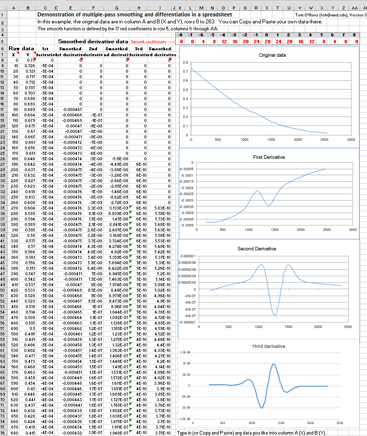In principle, it is possible to combine any degree of differentiation and smoothing into one set of shift-and-multiply coefficients (as illustrated here), but it's more flexible and easier to adjust if you compute the derivatives and each stage of smoothing separately in successive columns. This is illustrated by DerivativeSmoothing.ods for OpenOffice Calc and DerivativeSmoothing.xls for Excel (screen image), which smooths the data and computes the first derivative of Y (column B) with respect to X (column A), then applies that smoothing and differentiation process successively to compute the smoothed second and third derivatives. The same smoothing coefficients (in row 5, columns K through AA) are applied successively for each stage of differentiation; you can enter any set of numbers here (preferably symmetrical about the center number in column S). You can type or paste your own data into column A and B (X and Y), rows 8 to 263.

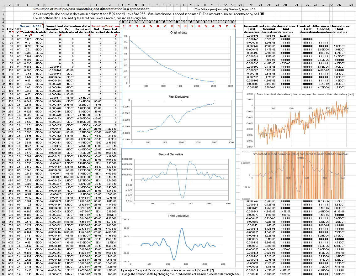
DerivativeSmoothingWithNoise.xlsx (graphic) demonstrates the dramatic effect of smoothing on the signal-to-noise ratio of derivatives on a noisy signal. It uses the same signal as DerivativeSmoothing.xls, but adds simulated white noise to the Y data. You can control the amount of added noise (cell D5).

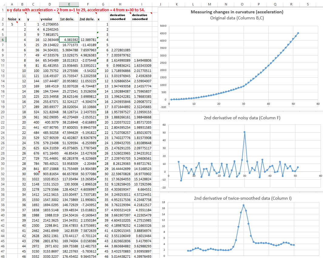
Another example of a derivative application is the spreadsheet SecondDerivativeXY2.xlsx (graphic), which demonstrates locating and measuring changes in the second derivative (a measure of curvature or acceleration) of a time-changing signal. This spreadsheet shows the apparent increase in noise caused by differentiation and the extent to which the noise can be reduced by smoothing (in this case by two passes of a 5-point triangular smooth). The smoothed second derivative shows a large peak the point at which the acceleration changes (at x=30) and plateaus on either side showing the magnitude of the acceleration before and after the change (y=2 and 4, respectively).

Differentiation in Matlab and Octave

Differentiation functions such as described above can easily be created in Matlab or Octave. Some simple derivative functions for equally-spaced time series data: deriv, a first derivative using the 2-point central-difference method, deriv1, an unsmoothed first derivative using adjacent differences,  deriv2, a second derivative using the 3-point central-difference method, a third derivative deriv3 using a 4-point formula, and deriv4, a 4th derivative using a 5-point formula. Each of these is a simple Matlab function of the form d=deriv(y); the input argument is a signal vector "y", and the differentiated signal is returned as the vector "d". For data that are not equally-spaced on the independent variable (x) axis, there are versions of the first and second derivative functions, derivxy and secderivxy, that take two input arguments (x,y), where x and y are vectors containing the independent and dependent variables. Click on these links to inspect the code, or right-click to download for use within Matlab. All of these are unsmoothed derivative that usually must be smoothed either after or before differentiation. Smoothed derivatives. Since smoothing almost always goes along with differentiation, the function SmoothDerivative.m combines the two. The syntax is  function Processed=SmoothedDerivative(x, y, DerivativeOrder, w, type, ends) where 'DerivativeOrder' determines the derivative order (0, 1, 2, 3, 4, 5), 'w' is the smooth width, 'type' determines the smooth mode:          If type=0, the signal is not smoothed.          If type=1, rectangular (sliding-average or boxcar)          If type=2, triangular (2 passes of sliding-average)          If type=3, pseudo-Gaussian (3 passes of sliding-average)          If type=4, Savitzky-Golay smooth and 'ends' controls how the "ends" of the signal (the first w/2 points and the last w/2 points) are handled          If ends=0, the ends are zeroed          If ends=1, the ends are smoothed with progressively smaller smooths the closer to the end. Peak detection. The simplest code to find peaks in x,y data sets simply looks for every y value that has lower y values on both sides (allpeaks.m). A alternative approach is to use the first derivative to find all the maxima by locating the points of zero-crossing, that is, the points at which the first derivative "d" (computed by derivxy.m) passes from positive to negative. In this example, the "sign" function is a built-in function that returns 1 if the element is greater than zero, 0 if it equals zero and -1 if it is less than zero. The routine prints out the value of x and y at each zero-crossing: d=derivxy(x,y); for j=1:length(x)-1    if sign(d(j))>sign(d(j+1))      disp([x(j) y(j)])    end end If the data are noisy, many false zero crossings will be reported; smoothing the data will reduce that. If the data are sparsely sampled, a more accurate value for the peak position (x-axis value at the zero crossing) can be obtained by interpolating between the point before and the point after the zero-crossing using the Matlab/Octave "interp1" function:  interp1([d(j) d(j+1)],[x(j) x(j+1)],0) ProcessSignal.m, a Matlab/Octave command-line function that performs smoothing and differentiation on the time-series data set x,y (column or row vectors). Type "help ProcessSignal". Returns the processed signal as a vector that has the same shape as x, regardless of the shape of y. The syntax is Processed=ProcessSignal(x, y, DerivativeMode, w, type, ends, Sharpen, factor1, factor2, SlewRate, MedianWidth) DerivativeDemo.m (shown above) is a self-contained Matlab/Octave demo function that uses ProcessSignal.m and plotit.m to demonstrate an application of differentiation to the quantitative analysis of a peak buried in an unstable background (e.g. as in various forms of spectroscopy). The object is to derive a measure of peak amplitude that varies linearly with the actual peak amplitude and is minimally effected by the background and the noise. To run it, just type DerivativeDemo at the command prompt. You can change several of the internal variables (e.g. Noise, BackgroundAmplitude) to make the problem harder or easier. Note that, despite the fact that the magnitude of the derivative seems to be numerically smaller than the original signal (because it has different units), the signal-to-noise ratio of the derivative is better and is much less effected by the background instability. (Execution time: 0.065 seconds in Matlab; 2.2 seconds in Octave). iSignal (shown above), and its Octave version isignaloctave.m, is an interactive multipurpose signal processing function for Matlab that includes differentiation and smoothing for time-series signals, up to the 5th derivative, automatically including the required type of smoothing. Simple keystrokes allow you to adjust the smoothing parameters (smooth type, width, and ends treatment) while observing the effect on your signal dynamically. In the example shown above, a series of three peaks at x=100, 250, and 400, with heights in the ratio 1:2:3, are buried in a strong curved background; the smoothed second and fourth derivatives are computed to suppress that background. View the code here or download the ZIP file with sample data for testing. (Version 2 of iSignal, November 2011, computes derivatives with respect to the x-axis vector, correcting for non-uniform x-axis intervals). These statements generate the 4th derivative of a Gaussian peak and display it in iSignal. You'll need to download isignal.m, gaussian.m, and deriv4.m. >> x=[1:.1:300]'; >> isignal(x,deriv4(100000.*gaussian(x,150,50)+.1*randn(size(x)))); The signal is mostly blue noise (because of the differentiated white noise) unless you smooth it considerately. Use the A and Z keys to increase and decrease the smooth width and the S key to cycle through the available smooth types. Hint: use the Gaussian smooth and keep increasing the smooth width. The script "iSignalDeltaTest" demonstrates the frequency response of the smoothing and differentiation functions of iSignal by a applying them to a delta function. Change the smooth type, smooth width, and derivative order and see how the power spectrum changes. Real-time differentiation in Matlab is discussed in Appendix Y   Data Differentiation Live Script DataDifferentiation.mlx is a Live Script for differentiation and smoothing applied to experimental data stored on disk. It is a variant of DataSmoothing.mlx discussed in the previous chapter, with the addition of a slider (in line 9) to select the derivative order (up to 10). The startpc and endpc sliders in lines 6 and 7 allow you to select which portion of the data range to display, from 0% to 100% of the total range of the data file. The other controls all relate to smoothing, which is especially important to improve the signal-to-noise ratio in differentiation. The smooth width (line 17) and the number of passes (line 18) are important. The general rule is: for the nth derivative, set the number of passes to at least n+1. Note: If the "PlotBeforeAndAfter" check box is checked, the derivative (red curve) will be scaled to match the maximum of the original signal (black curve). If that box is not checked, the derivative will be displayed by itself with its actual amplitude. (This is done because the numerical amplitudes of derivative is often orders of magnitude different than the original signals). .

created and maintained by Prof. Tom O'Haver , Professor Emeritus, Department of Chemistry and Biochemistry, The University of Maryland at College Park. Comments, suggestions and questions should be directed to Prof. O'Haver at toh@umd.edu.