Toolkit of functions, scripts and spreadsheet templates

for "A Pragmatic Introduction to Signal Processing"

[Peak shape functions]  [Signal arithmetic]  [Signals and noise]  [Smoothing]  [Differentiation and peak sharpening]  [Harmonic analysis]  [Fourier convolution and deconvolution]  [Fourier filter]  [Wavelets]  [Peak area measurement]  [Linear Least Squares]  [Peak Finding and Measurement] [Multicomponent Spectroscopy]  [Iterative Curve Fitting]  [Hyperlinear quantitative absorption spectroscopy]   [MAT and txt files] [Spreadsheet templates for Microsoft Excel and OpenOffice Calc]

The is a list of all the functions, scripts, data files, and spreadsheets used in this essay. You can right-click and select "Save link as..." to download them to your computer. There are approximately 200 Matlab/Octave m-files (functions and demonstration scripts); place these into the Matlab or Octave "path" so you can use them just like any other built-in feature. (Difference between scripts and functions). To display the built-in help for these functions and script, type "help <name>" at the command prompt (where "<name>" is the name of the script or function).

Items marked or on this page are recently added within the past year or so.

Spreadsheet files are available in .xls format for Excel, but they can also be opened in OpenOffice Calc.

If you are unsure whether you have all the latest versions, the simplest way to update all my functions, scripts, tools, spreadsheets and documentation files is to download the latest site archive ZIP file (approx. 200 MBytes), then right-click on the zip file and click "Extract all". Then list the contents of the extracted folder by date and then drag and drop any new or newly updated files into a folder in your Matlab/Octave path. The ZIP files contains all the files used by this web site in one directory, so you can search for them by file name or sort them by date to determine which ones that have changed since the last time you downloaded them.

If you try to run one of my scripts or functions and it gives you a "missing function" error, look for the missing item here, download it into your path, and try again. The script testallfunctions.m is intended to test for the existence of all/most of the functions in this collection. If it comes to a function that is not installed on your system, or if one of them does not run, it will stop with an error, alerting you of the problem. It takes about 5 minutes to run in Matlab on a contemporary PC (slower in Octave).
 
Some of these functions have been requested by users, suggested by Google search terms, or corrected and expanded based on extensive user feedback; you could almost consider this an international "crowd-sourced" software project. I wish to express my thanks and appreciation for all those who have made useful suggestions, corrected errors, and especially those who have sent me data from their work to test my programs on. These contributions have really helped to correct bugs and to expand the capabilities of my programs.

Peak shape functions (for Matlab and Octave)

Most of these shape functions take three required input arguments: the independent variable ("x") vector, the peak position, "pos", and the peak width, "wid", usually the full width at half maximum. The functions marked 'variable shape' require an additional fourth input argument that determines the exact peak shape. The sigmoidal and exponential shapes (alpha function, exponential pulse, up-sigmoid, down-sigmoid, Gompertz, FourPL, and OneMinusExp) have different input argument variables names.

Gaussian y = gaussian(x,pos,wid)
exponentially-broadened Gaussian (variable shape)
Triangle-broadened Gaussian (variable shape)
bifurcated Gaussian (variable shape)
Flattened Gaussian (variable shape)
Clipped Gaussian (variable shape)
Lorentzian (aka 'Cauchy') y = lorentzian(x,pos,wid)
exponentially-broadened Lorentzian (variable shape)
Clipped Lorentzian (variable shape)
Gaussian/Lorentzian blend (variable shape)
Voigt profile (variable shape)
lognormal
logistic distribution (for logistic function, see up-sigmoid)
Pearson 5 (variable shape)
alpha function
exponential pulse
sech2, a peak shape intermediate between Gaussian and Lorentzian. See Sech2ShapeComparison.m (graphic).
plateau (variable shape, symmetrical product of sigmoid and down sigmoid, similar to Flattened Gaussian)
Breit-Wigner-Fano resonance (BWF) (variable shape)
triangle
exponentially-broadened triangle (variable shape)
Gaussian/Triangle blend (variable shape)
 rectanglepeak
tsallis distribution (variable shape, similar to Pearson 5)
up-sigmoid (logistic function or "S-shaped"). Simple upward going sigmoid.
down-sigmoid ("Z-shaped") Simple downward going sigmoid.
Gompertz, 3-parameter logistic, a variable-shape sigmoidal:
y=Bo*exp(-exp((Kh*exp(1)/Bo)*(L-t) +1))
FourPL, 4-parameter logistic, y = maxy+(miny-maxy)./(1+(x./ip).^slope)
OneMinusExp, Asymptotic rise to flat plateau: g = 1-exp(-wid.*(x-pos))
peakfunction.m, a function that generates many different peak types specified by number.

modelpeaks, a function that simulates multi-peak time-series signal data consisting of any number of peaks of the same shape. Syntax is model= modelpeaks(x, NumPeaks, peakshape, Heights, Positions, Widths, extra), where 'x' is the independent variable vector, 'NumPeaks' in the number of peaks, 'peakshape' is the peak shape number, 'Heights' is the vector of peak heights, 'Positions' is the vector of peak positions,'Widths' is the vector of peak widths, and 'extra' is the additional shape parameter required by the exponentially broadened, Pearson, Gaussian/Lorentzian blend, BiGaussian and BiLorentzian shapes. Type 'help modelpeaks'. To create noisy peaks, use one of the following noise functions to create some random noise to add to the modelpeaks array.

modelpeaks2, a function that simulates multi-peak time-series signal data consisting of any number of peaks of different shapes. Syntax is y=modelpeaks2(t, Shape, Height, Position, Width, extra)where 'shape' is a vector of peak type numbers and the other input arguments are the same as for modelpeaks.m. Type 'help modelpeaks2'

ShapeDemo demonstrates 16 basic peak shapes graphically, showing the variable-shape peaks as multiple lines.

SignalGenerator.m is a script to create and plot realistic computer-generated signal consisting of multiple peaks on a variable baseline plus variable random noise. You may change the lines here marked by <<< to modify the character of the signal peaks, baseline, and noise.

Signal Arithmetic

stdev.m Octave and Matlab compatible standard deviation function (because the regular built-in std.m function behaves differently in Matlab and in Octave). rsd.m is the relative standard deviation (the standard deviation divided by the mean). prsd.m is the percent relative standard deviation (100 times the relative standard deviation).

PercentDifference.m A simple function that calculates the percent difference between two numbers or vectors, i.e. 100*(b-a)/a, where a and b can be scalar or vector.

val2ind(x,val) Returns the index and the value of the element of vector x that is closest to "val". If more than one element is equally close, returns vectors of indicies and values, Example:  If x=[1 2 4 3 5 9 6 4 5 3 1], then val2ind(x,6)=7 and val2ind(x,5.1)=[5 9]. This is useful for accessing subsets of x,y data sets; for example,  the code sequence x1=7; x2=8; irange=val2ind(x,x1):val2ind(x,x2); xx=x(irange); yy=y(irange); plot(xx,yy) will plot x vs y only over the range of x values from 7 to 8. See also PeakFindingandMeasurement.htm#UsingP

halfwidth and tenthwidth: [FWHM,slope1,slope2,hwhm1,hwhm2] = halfwidth(x,y,xo) uses linear interpolation between points to compute the approximate FWHM (full width at half maximum) of any smooth peak whose maximum is at x=xo, has a zero baseline, and falls to below one-half of the maximum height on both sides. Not accurate if the peak is noisy or sparsely sampled. If the additional output arguments are supplied, it also returns the leading and trailing edge slopes, slope1 and slope2, and the leading and trailing edge half widths at half maximum, hwhm1 and hwhm2, respectively. If x0 is omitted, it determines the halfwidth of the largest peak. Example: xo=500; width=100; x=1:1000; y=exp(-1.*((x-xo)/(0.60056120439323.*width)).^2); halfwidth(x,y,xo). The analogous function [twidth,slope1,slope2,hwhm1,hwhm2] = tenthwidth(x,y,xo) computes the full width at 1/10 maximum, and just for the heck of it, hundredthwidth, [hwidth,slope1,slope2] = hundredthwidth(x,y,xo), computes the full width at 1/100 maximum.

MeasuringWidth.m is a script that compares two methods of measuring the full width at half maximum of a peak: gaussian fitting (using peakfit.m) and direct interpolation (using halfwidth.m). The two methods agree exactly for a finely-sampled noiseless Gaussian on a zero baseline, but give slightly different answers if any of these conditions are not met. The halfwidth function works well for any finely-sampled smooth peak shape on a zero baseline, but the peakfit function is better at resisting random noise and it has the ability to correct for some types of baseline and it has a wide selection of peak shapes to use as a model. See the help file.

IQrange.m, estimates the standard deviation of a set of numbers by dividing its "interquartile range" (IQR) by 1.34896, an alternative to the usual standard deviation calculation that works better for computing the dispersion (spread) of a data set that contains outliers. Essentially it's the standard deviation with outliers removed. Syntax is b = IQrange(a).

rmnan(a) "ReMoveNotANumber". Removes NaNs ("Not a Number") and Infs (" Infinite") from vectors, replacing with nearest real numbers and printing out the number of changes (if any are made). Use this to prevent subsequent operations from stopping on an error.

rmz(a) ReMoves Zeros from vectors, replacing with nearest non-zero numbers and printing out the number of changes (if any are made). Use this to remove zeros from vectors that will subsequently be used as the denominator of a division.

[a,changes]=nht(a,b); "no higher than" replaces any numbers in vector a that are greater than the scalar b with b. Optionally "changes" returns the number of changes.

[a,changes]=nlt(a,b); "no lower than" replaces any numbers in vector a that are less than the scalar b with b. Optionally "changes" returns the number of changes.

makeodd(a): Makes the elements of vector "a" the next higher odd integers. This can be useful in computing smooth widths to insure that the smooth will not shift the maximum of peaks.  For example, makeodd([1.1 2 3 4.8 5 6 7.7 8 9]) = [1 3 3 5 5 7 9 9 9]

condense(y,n), function to reduce the length of vector y by replacing each group of n successive values by their average. The similar function condensem.m works for matrices. Use to re-sample an oversampled signal. Mentioned on Smoothing.html and iSignal.html.

val2ind(x,val), returns the index and the value of the element of vector x that is closest to val. Example: if x=[1 2 4 3 5 9 6 4 5 3 1], then val2ind(x,6)=7 and val2ind(x,5.1)=[5 9]. For some examples of how this can be used, see PeakFindingandMeasurement.htm#UsingP and InteractivePeakFitter.htm#FitResultsTable. testcondense.m is a script that demonstrates of the effect of boxcar averaging using the condense.m function to reduce noise without changing the noise color. Shows that it reduces the measured noise, removing the high frequency components, resulting in a faster fitting execution time and a lower fitting error, but no more accurate measurement of peak parameters.

NumAT(m,threshold): "Numbers Above Threshold": Counts the number of adjacent elements in the vector 'm' that are greater than or equal to the scalar value 'threshold'. Returns a matrix listing each group of adjacent values, their starting index, the number of elements in that group, and the sum of that group, and the mean. Type "help NumAT" and try the example.

isOctave.m  Returns 'true' if this code is being executed by Octave. Returns 'false' if this code is being executed by MATLAB, or any other MATLAB variant. Useful in those few cases where there is a small difference between the syntax or operation of Matlab and Octave functions, as for example trypoly(x,y), tablestats.m, and trydatatrans.m.

Data plotting. The Matlab/Octave scripts plotting.m and plotting2.m show how to plot multiple signals using matrices and subplots (multiple small plots in a single Figure window). The scripts realtimeplotautoscale.m and realtimeplotautoscale2.m demonstrating plotting in real time (animated graphic).

plotit, version 2, (previously named 'plotfit'), is an easy-to-use function for plotting x,y data in matrices or in separate vectors. Syntax:  [coef,RSquared,StdDevs,BootResults] = plotit(xi,yi,polyorder,datastyle,fitstyle). It can also fit polynomials to the data and compute errors. Click here or type "help plotit" at the Matlab/Octave prompt for examples.

Signals and Noise

whitenoise, pinknoise, bluenoise propnoise, sqrtnoise, bimodal: different types of random noise that might be encountered in physical measurements. Type "help whitenoise", etc, for help and examples.

noisetest.m is a self-contained Matlab/Octave function for demonstrating different noise types. It plots Gaussian peaks with four different types of added noise with the same standard deviation: constant white noise; constant pink (1/f) noise; proportional white noise; and square-root white noise, then fits a Gaussian model to each noisy data set and computes the average and the standard deviation of the peak height, position, width and area for each noise type. See SignalsAndNoise.html. Se also NoiseColorTest.m.

SubtractTwoMeasurements.m is a Matlab/Octave script demonstration of measuring the noise and signal-to-noise ratio of a stable waveform by subtracting two measurements of the signal waveform, m1 and m2 and computing the standard deviation of the difference The signal must be stable between measurements (except for the random noise). The standard deviation of the measured noise is given by sqrt((std(m1-m2)²)/2).

NoiseColorTest.m, a function that demonstrates the effect of smoothing white, pink, and blue noise. It displays a graphic of 5 noise color types both before and after smoothing, as well as their frequency spectra. All noise samples have a standard deviation of 1.0 before smoothing. You can change the smooth width and type in lines 6 and 7.

CurvefitNoiseColorTest.m, a function that demonstrates the effect of white, pink, and blue noise on curve fitting a single Gaussian peak.

RANDtoRANDN.m is a script that demonstrates how the expression 1.73*(RAND() - RAND() + RAND() - RAND()) approximates normally-distributed random numbers with zero mean and a standard deviation of 1. See SignalsAndNoise.html.

RoundingError.m. A script that demonstrates digitization (rounding) noise and shows that adding noise and then ensemble averaging multiple signals can reduce the overall noise in the signal. A rare example where adding noise is actually beneficial. See CaseStudies.html#Digitization.

DigitizedSpeech.m, an audible/graphic demonstration of rounding error on digitized speech. It starts with an audio recording of the spoken phrase "Testing, one, two, three", previously recorded at 44000 Hz and saved in WAV format (download link), rounds off the amplitude data progressively to 8 bits (256 steps), 4 bits (16 steps), and 1 bit (2 steps), and then the same with random white noise added before the rounding (2 steps + noise), plots the waveforms and plays the resulting sounds, demonstrating both the degrading effect of rounding and the remarkable improvement caused by adding noise. See CaseStudies.html#Digitization.

CentralLimitDemo.m, script that demonstrates that the more independent uniform random variables are combined, the probability distribution becomes closer and closer to normal (Gaussian). See SignalsAndNoise.html.

EnsembleAverageDemo.m is a Matlab/Octave script that demonstrates ensemble averaging to improved the signal-to-noise ratio of a very noisy signal. Click for graphic. The script requires the "gaussian.m" function to be downloaded and placed in the Matlab/Octave path, or you can use any other peak shape function, such as lorentzian.m or rectanglepulse.m.

EnsembleAverageDemo2.m is a Matlab/Octave script that demonstrates the effect of amplitude noise, frequency noise, and phase noise on the ensemble averaging of a sine waveform.

EnsembleAverageFFT.m is a Matlab/Octave script that demonstration of the effect of amplitude noise, frequency noise, and phase noise on the ensemble averaging of a sine waveform signal. Shows that: (a) ensemble averaging reduces the white noise in the signal but not the frequency or phase noise, (b) ensemble averaging the Fourier transform has the same effect as ensemble averaging the signal itself, and (c) the effect of phase noise is reduced if the power spectra are ensemble averaged. EnsembleAverageFFTGaussian.m does the same for a Gaussian peak signal, where variation in peak width is frequency noise and variation in peak position is phase noise.

iPeakEnsembleAverageDemo.m ia a self-contained demonstration of the iPeak function. In this example, the signal contains a repeated pattern of two overlapping Gaussian peaks of width 12, with a 2:1 height ratio. These patterns occur a random intervals, and the noise level is about 10% of the average peak height. Using iPeak's ensemble average function (Shift-E), the patterns can be averaged and the signal-to-noise ratio significantly improved. See CaseStudies.html#Ensemble.

PeriodicSignalSNR.m is a Matlab/Octave script demonstrating the estimation of the peak-to-peak and root-mean-square signal amplitude and the signal-to-noise ratio of a periodic waveform, estimating the noise by looking at the time periods where its envelope drops below a threshold. See CaseStudies.html#SNR.

iPeakEnsembleAverageDemo.m is a demonstration of iPeak's ensemble average function. In this example, the signal contains a repeated pattern of two overlapping Gaussian peaks, 12 points apart, both of width 12, with a 2:1 height ratio. These patterns occur a random intervals throughout the recorded signal, and the random noise level is about 10% of the average peak height. Using iPeak's ensemble average function (Shift-E), the patterns can be averaged and the signal-to-noise ratio significantly improved.

LowSNRdemo.m is a script that compares several different methods of peak measurement with very low signal-to-noise ratios. It creates a single peak, with adjustable shape, height, position, and width, adds constant white random noise so the signal-to-noise ratio varies from 0 to 2, then measures the peak height and position by each method and computes the average error. Four methods are compared: (1) the peak-to-peak measure of the smoothed signal and background; (2) a peak finding method based on findpeakG; (3) unconstrained iterative least-squares fitting (INLS) based on the peakfit.m function; and (4) constrained classical least squares fitting (CLS) based on the cls2.m function. See Appendix J: How Low can you Go? Performance with very low signal-to-noise ratios.

RandomWalkBaseline.m simulates a Gaussian peak with randomly variable position and width superimposed on a drifting "random walk" baseline. Compare to WhiteNoiseBaseline.m. See CaseStudies.html#RandomWalk.

AmplitudeModulation.m is a Matlab/Octave script simulation of modulation and synchronous detection, demonstrating the noise reduction capability. See CaseStudies.html#Modulation.

DerivativeNumericalPrecisionDemo.m. Self-contained function that demonstrates how the numerical precision limits of the computer effects the first through fourth derivatives of a smooth ("noiseless") Gaussian band, showing both the waveforms (in Figure 1) and their frequency spectra (in Figure 2). The numerical precision limit of the computer creates random noise at very high frequencies, which is emphasized by differentiation, and by the fourth derivative that noise overwhelms the signal frequencies at lower frequencies. Smoothing with a Gaussian (three passes of a sliding-average) smooth with a smooth ratio of 0.2 removes most of the noise. With real experimental data, even the tiniest amounts of noise in the original data would be much greater than this. Used in CaseStudies.html#Numerical.

RegressionNumericalPrecisionTest.m is a Matlab/Octave script that demonstrates how the numerical precision limits of the computer effects the Classical Least Squares (multilinear regression) of two very closely-spaced "noiseless" overlapping Gaussian peaks. This uses three different mathematical formulation of the least-squares calculation that give different results when the numerical precision limits of the computer are reached. But practically, the difference between these methods is unlikely to be seen; even the tiniest bit of added random noise (line 15) or signal instability produces a far greater error. Used in CaseStudies.html#Numerical.

RegressionADCbitsTest.m. Demonstration of the effect of analog-to-digital converter resolution (defined by the number of bits in line 9) on Classical Least Squares (multilinear regression) of two closely-spaced overlapping Gaussian peaks. Normally, the random noise (line 10) produces a greater error than the ADC resolution. Used in CaseStudies.html#Numerical.

Smoothing

fastsmooth, versatile function for fast data smoothing. The syntax is SmoothY=fastsmooth(Y,w,type,ends). See Smoothing.html#Matlab. Note: Greg Pittam has published a modification of the fastsmooth function that tolerates NaNs (Not a Number) in the data file (nanfastsmooth(Y,w,type,tol)) and a version for smoothing angle data (nanfastsmoothAngle(Y,w,type,tol)). Click for animated example.

SegmentedSmooth.m, segmented multiple-width data smoothing function based on the fastsmooth algorithm. The syntax is SmoothY = SegmentedSmooth(Y,smoothwidths,type,ends). This function divides Y into a number of equal-length segments according to the length of the vector 'smoothwidths', then smooths each segment with a smooth of width defined by the sequential elements of vector 'smoothwidths' and smooth type 'type'. Type "help SegmentedSmooth" for examples. DemoSegmentedSmooth.m demonstrates the operation (click for graphic). See CaseStudies.html#Segmented.

medianfilter , median-based filter function for eliminating narrow spike artifacts. The syntax is mY=medianfilter(y,Width), where "Width" is the number of points in the spikes that you wish to eliminate. Type "help medianfilter" at the command prompt.

killspikes.m is a threshold-based filter function for eliminating narrow spike artifacts. The syntax is fy= killspikes(x, y, threshold, width). Each time it finds a positive or negative jump in the data between y(n) and y(n+1) that exceeds "threshold", it replaces the next "width" points of data with a linearly interpolated segment spanning x(n) to x(n+width+1), See killspikesdemo. Type "help killspikes" at the command prompt.

testcondense.m is a script that demonstrates of the effect of boxcar averaging using the condense.m function, which performs a non-overlapping boxcar averaging function, to reduce noise without changing the noise color. Shows that it reduces the measured noise, removing the high frequency components, resulting in a faster fitting execution time and a lower fitting error, but unfortunately no more accurate measurement of peak parameters.

SmoothWidthTest.m is a Matlab/Octave script that demonstrates the effect of smoothing on the peak height, random white noise, and signal-to-noise ratio of a noisy peak signal. Produces an animation showing the effect of progressively wider smooth widths, then draws a graph of peak height, noise, and signal-to-noise ratio vs smooth ratio. Click to see gif animation. You can change the peak shape and width in line 8 and the smooth type in line 9: 1=rectangle; 2=triangle; 3=pseudo Gaussian. The script requires the "gaussian.m" function to be downloaded and placed in the Matlab/Octave path, or you can use any other peak shape function, such as lorentzian.m or rectanglepulse.m, etc.

SmoothExperiment.m, very simple script that demonstrates the effect of smoothing on the position, width, and height of a single Gaussian peak. Requires that the fastsmooth.m and peakfit.m functions be present in the path. See Smoothing.html#Matlab

smoothdemo.m compares the performance and speed of four types of smooth operations: (1) sliding-average, (2) triangular, (3) pseudo-Gaussian (equivalent to three passes of a sliding-average), and (4) Savitzky-Golay. These smooth operations are applied to a single noisy Gaussian peak. The peak height of the smoothed peak, the standard deviation of the smoothed noise, and the signal-to-noise ratio are all measured as a function of smooth width. See Smoothing.html#Matlab. The modified script, smoothdemoWavelet.m adds wavelet denoising as method #5 (requires the Wavelet Toolkit).

SmoothOptimization.m, script that shows why you don't need to smooth data prior to least-squares curve fitting; it compares the effect of smoothing on the signal-to-noise ratio of peak height of a noisy Gaussian peak, using three different measurement methods. Requires that the fitgauss2.m, gaussfit.m, gaussian.m, and fminsearch.m functions be present in the path. See CurveFittingC.html#Smoothing.

SmoothVsCurvefit.m, comparison of peak height measurement by taking the maximum of the smoothed signal and by curve fitting the original unsmoothed data. Requires peakfit.m and gaussian.m in path.

DemoSegmentedSmooth.m demonstrates the operation of SegmentedSmooth.m with a signal consisting of noisy variable-width peaks that get progressively wider. Requires SegmentedSmooth.m and gaussian.m in the path.

DeltaTest.m. A simple Matlab/Octave script that demonstrates the shape of any smoothing algorithm can be determined by applying that smooth to a delta function, a signal consisting of all zeros except for one point.

iSignal performs several different kinds of smoothing, segmented smoothing, median filtering, and spike removal (as well as differentiation, peak sharpening, least-squares measurements of peak position, height, width, and area, signal and noise amplitudes, frequency spectra in selected regions of the signal, and signal-to-noise ratio of peaks). m-file link: isignal.m. Click here to download the ZIP file "iSignal6.zip". Click for animated example.

The script RealTimeSmoothTest.m demonstrates real-time smoothing, plotting the raw unsmoothed data as a black line and the smoothed data in red. In this case the script pre-calculates simulated data in line 28 and then accesses the data point-by-point in the processing loop (lines 30-51). The total number of data points is controlled by 'maxx' in line 17 (initially set to 1000) and the smooth width (in points) is controlled by 'SmoothWidth' in line 20. Animated graphic.

Data Smoothing Tool (download link: DataSmoothing.mlx) is an interactive Live Script that can apply several types of smoothing to experimental data stored on disk. It can perform spike removal, sliding average smooths with up to 5 passes, Savitsky-Golay and Fourier low-pass filtering, and wavelet denoising (which requires the Matlab Wavelet Toolkit).

Differentiation and peak sharpening

deriv, deriv2, deriv3, deriv4, derivxy and secderivxy, simple functions for computing the derivatives of time-series data. See Differentiation.html#Matlab

 SmoothDerivative.m combines differentiation and smoothing. The syntax is SmoothedDeriv = SmoothedDerivative(x,y,DerivativeOrder,w,type,ends) where 'DerivativeOrder' determines the derivative order (0, 1, 2, 3, 4, 5), 'w' is the smooth width, 'type' determines the smooth mode:
         If type=0, the signal is not smoothed.
         If type=1, rectangular (sliding-average or boxcar)
         If type=2, triangular (2 passes of sliding-average)
         If type=3, pseudo-Gaussian (3 passes of sliding-average)
         If type=4, Savitzky-Golay smooth
and 'ends' controls how the "ends" of the signal (the first w/2 points and the last w/2 points) are handled
         If ends=0, the ends are zeroed
         If ends=1, the ends are smoothed with progressively smaller smooths the closer to the end.
Type "help SmoothDerivative" for some examples (graphic).

SlopeAnimation.m is an animated Matlab/Octave demonstration that shows that the first derivative of a signal is the slope of the tangent to the signal at each point.

DataDifferentiation.mlx is a Live Script tool for differentiation.

sharpen, Resolution enhancement (peak sharpening) by the even-derivative method. Syntax is SharpenedSignal= sharpen(signal, factor1, factor2, SmoothWidth). See ResolutionEnhancement.html. Related demos: SegmentedSharpen.m, DemoSegmentedSharpen.m (graphic), SharpenedGaussianDemo.m (graphic), SharpenedGaussianDemo4terms.m (graphic), SharpenedLorentzianDemo.m (graphic), SharpenedLorentzianDemo4terms.m.  The script SharpenedOverlapDemo.m (graphic) demonstrates the effect of sharpening on perpendicular drop area measurements of two overlapping Gaussians peaks with adjustable height, separation, and width, calculating the percent different between the area measured on the overlapping peak signal compared to the true areas of the isolated peaks. SharpenedOverlapDemo.m is a script that automatically determines the optimum degree of even-derivative sharpening that minimizes the errors of measuring peak areas of two overlapping Gaussians by the perpendicular drop method using the autopeaks.m function. (Graphic 1, Graphic 2).

ProcessSignal, a Matlab/Octave command-line function that performs smoothing, See differentiation, peak sharpening, and median filtering on the time-series data set x,y (column or row vectors). Similar to iSignal, without the plotting and interactive keystroke controls. Type "help ProcessSignal". Returns the processed signal as a vector that has the same shape as x, regardless of the shape of y. The syntax is Processed= ProcessSignal(x, y, DerivativeMode, w, type, ends, Sharpen, factor1, factor2, SlewRate, MedianWidth).

derivdemo1.m, a function that demonstrates the basic shapes of derivatives. See Differentiation.html#BasicProperties

DerivativeShapeDemo.m is a function that demonstrates the first derivatives of 16 different peak shapes. (graphic)

derivdemo2.m, a function that demonstrates the effect of peak width on the amplitude of derivatives. See Differentiation.html#BasicProperties

derivdemo3.m, a function that demonstrates the effect of smoothing on the first derivative of a noisy signal. See Differentiation.html#Smoothing

derivdemo4.m, a function that demonstrates the effect of smoothing on the second derivative of a noisy signal. See Differentiation.html#Smoothing

DerivativeDemo.m is a self-contained Matlab/Octave demo function that uses ProcessSignal.m and plotit.m to demonstrate an application of differentiation to the quantitative analysis of a peak buried in an unstable background (e.g. as in various forms of spectroscopy). The object is to derive a measure of peak amplitude that varies linearly with the actual peak amplitude and is minimally effected by the background and the noise. To run it, just type DerivativeDemo at the command prompt. You can change several of the internal variables (e.g. Noise, BackgroundAmplitude) to make the problem harder or easier. Note that, despite the fact that the magnitude of the derivative is numerically smaller than the original signal (because it has different units), the signal-to-noise ratio of the derivative is better, and the derivative signal is linearly proportional to the actual peak height, despite the interference of large background variations and random noise. See Differentiation.html

iSignal is an interactive function for Matlab that performs differentiation, smoothing, and peak sharpening for time-series signals, up to the 5^th derivative, automatically including the required type of smoothing. Simple keystrokes allow you to adjust the smoothing and sharpening parameters while observing the effect on your signal dynamically. Click here to download the ZIP file "iSignal7.zip". Click for animated example. Version 7, June 2019, includes the ability to symmetrize exponentially broadened peaks peaks by weighted first derivative addition.

demoisignal.m for Matlab is a self-running script that demonstrates the features of iSignal (and requires that the latest version of iSignal, and version 6 of plotit.m, be present in your Matlab path). Demonstrates panning and zooming, smoothing, differentiation, frequency spectrum, peak measurement, and derivative spectroscopy calibration (in conjunction with plotit.m version 6).

iSignalDeltaTest is a Matlab/Octave script that demonstrates the frequency response (power spectrum) of the smoothing and differentiation functions of iSignal by a applying them to a delta function. Change the smooth type, smooth width, and derivative order and see how the power spectrum changes.

 The script RealTimeSmoothFirstDerivative.m demonstrates real-time smoothed differentiation, using a simple adjacent-difference algorithm (line 47) and plotting the raw data as a black line and the first derivative data in red. The script RealTimeSmoothSecondDerivative.m computes the smoothed second derivative by using a central difference algorithm (line 47). Both of these scripts pre-calculate the simulated data in line 28 and then accesses the data point-by-point in the processing loop (lines 31-52).  In both cases the maximum number of points is set in line 17 and the smooth width is set in line 20.

 The script RealTimePeakSharpening.m demonstrates real-time peak sharpening using the second derivative technique. It uses pre-calculated simulated data in line 30 and then accesses the data point-by-point in the processing loop (lines 33-55). In both cases the maximum number of points is set in line 17 and the smooth width is set in line 20 and the weighting factor (K1) is set in line 21. In this example the smooth width is 101 points, which accounts for the the delay in the sharpened peak compared to the original.

Harmonic Analysis

FrequencySpectrum.m (syntax fs=FrequencySpectrum(x,y)) returns a matrix containing the real part of the Fourier power spectrum of x,y. To plot it, type "plotit(fs)". Input data can be separate x and y vectors of both in a matrix. Type "help FrequencySpectrum".

PlotFrequencySpectrum.m plots the frequency spectrum or periodogram of the signal x,y on linear or log coordinates. The syntax is PowerSpectrum= PlotFrequencySpectrum(x, y, plotmode, XMODE, LabelPeaks). Type "help PlotFrequencySpectrum" for details. Try this example:
x= [0:.01:2*pi]'; y=sin(200*x)+randn(size(x));
subplot(2,1,1); plot(x,y); subplot(2,1,2); PowerSpectrum=PlotFrequencySpectrum(x,y,1,0,1);

CompareFrequencySpectrum.m. A script that compares two signals (upper panel) and their frequency spectra (lower panel) with the original signal shown in blue and the modified signal in green. plotmode: =1:linear, =2:semilog X, =3:semilog Y; =4: log-log). XMODE: =0 for frequency Spectrum (x is frequency); =1 for periodogram (x is time). Define the signal modification in line 15. You can load a signal stored in .mat format or create an simulated signal for testing. Must have PlotFrequencySpectrum.m in the path.

PlotSegFreqSpect.m plots and segmented Fourier spectrum (syntax PSM=(x,y,NumSegments,MaxHarmonic,LogMode)). It breaks y into 'NumSegments' equal length segments, multiplies each by an apodizing window function, computes the power spectrum of each segment, returns the power spectrum matrix (PSM), and plots the result of the first 'MaxHarmonic' Fourier components as as a contour plot. See HarmonicAnalysis.html#Software

SineToDelta.m. A demonstration animation (animated graphic) showing the waveform and the power spectrum of a rectangular pulsed sine wave of variable duration (whose power spectrum is a "sinc" function) changing continuously from a pure sine wave at one extreme (where its power spectrum is a delta function) to a single-point pulse at the other extreme (where its power spectrum is a flat line). GaussianSineToDelta.m is similar, except that it shows a Gaussian pulsed sine wave, whose power spectrum is a Gaussian function, but which is the same at the two extremes of pulse duration (animated graphic).

iSignal is a multi-purpose interactive signal processing tool (for Matlab only) that includes a Frequency Spectrum mode, toggled on and off by the Shift-S key; it computes frequency spectrum of the segment of the signal displayed in the upper window and displays it in the lower window (in red). You can use the pan and zoom keys to adjust the region of the signal to be viewed or press Ctrl-A to select the entire signal. Press Shift-S again to return to the normal mode. See CaseStudies.html#Harmonic for a relevant example. Click for animated example.

iPower, a keyboard-controlled interactive power spectrum demonstrator, useful for teaching and learning about the power spectra of different types of signals and the effect of signal duration and sampling rate. Single keystrokes allow you to select the type of signal (12 different signals included), the total duration of the signal, the sampling rate, and the global variables f1 and f2 which are used in different ways in the different signals. When the Enter key is pressed, the signal (y) is sent to the Windows WAVE audio device. Press K to see a list of all the keyboard commands. (m-file link: ipower.m). Slideshow of examples.

The script RealTimeFrequencySpectrumWindow.m computes and plots the Fourier frequency spectrum of a signal. It loads the simulated real-time data from a ".mat file" (in line 31) and then accesses that data point-by-point in the processing 'for' loop. A critical variable in this case is "WindowWidth" (line 37), the number of data points taken to compute each frequency spectrum. If the data stream is an audio signal, it's also possible to play the sound through the computer's sound system synchronized with the display of the frequency spectra (set "PlaySound" to 1).

Fourier convolution and deconvolution

ExpBroaden, exponential broadening function. Syntax is yb = ExpBroaden(y,t). Convolutes the vector y with an exponential decay of time constant t. Mentioned on SignalsAndNoise.html and InteractivePeakFitter.htm.

GaussConvDemo.m, a script that demonstrates that a Gaussian of unit height, Fourier convoluted with a centered Gaussian of the same width is a shorter, broader Gaussian (with a height of 1/sqrt(2) and a width of sqrt(2) and of equal area to the original Gaussian). The bottom panel shows an attempt to recover the original y from the convoluted result. You can optionally add noise  to show how convolution smooths the noise and how Fourier deconvolution restores it. Requires gaussian.m in path.

CombinedDerivativesAndSmooths.txt. Convolution coefficients for computing the first through fourth derivatives, with rectangular, triangular and Gaussian smooths.

Convolution.txt, simple examples of whole-number convolution vectors for smoothing and differentiation.

deconvolutionexample.m, a simple example script that demonstrates the use of the Matlab Fourier deconvolution 'deconv' function. See Deconvolution.html.

DeconvDemo.m, a Fourier deconvolution demo script with a signal containing four Gaussians broadened by an exponential function (graphic). DeconvDemo2.m is a similar script for a single Gaussian (graphic). DeconvDemo3.m demonstrates deconvolution of a Gaussian convolution function from a rectangular pulse (animated graphic). DeconvDemo4.m (animated graphic) demonstrates "self deconvolution" applied a signal consisting of a Gaussian peak that is broadened by the measuring instrument, and an attempt to recover the original peak width.  DeconvDemo5.m (graphic) shows an attempt to resolve two closely-spaced underlying peaks that are completely unresolved in the observed signal. See CaseStudies.html#deconvolution. Variation of this include versions with Lorentzian peaks and one with a triangular convolution function.

deconvgauss.m. function ydc=deconvgauss(x,y,w) deconvolutes a Gaussian function of width 'w' from vector y, returning the deconvoluted result.

deconvexp.m. function ydc=deconvexp(y,tc) deconvolutes an exponential function of time constant 'tc' from vector y, returning the deconvoluted result.

SegExpDeconv(x,y,tc) is a segmented version of deconvexp.m; it divides x,y into a number of equal-length segments defined by the length of the vector 'tc', then each segment is deconvoluted with an exponential decay of the form exp(-x./t) where t is corresponding element of the vector tc. Any number and sequence of t values can be used. Useful when the peak width and/or exponential tailing of peaks varies across the signal duration. SegExpDeconvPlot.m is the same except that it plots the original and deconvoluted signals and shows the divisions between the segments by vertical magenta lines. SegGaussDeconv.m and SegGaussDeconvPlot.m are the same except that they perform a symmetrical (zero-centered) Gaussian deconvolution. SegDoubleExpDeconv.m and SegDoubleExpDeconvPlot.m perform a symmetrical (zero-centered)exponential deconvolution.

 iSignal has a Shift-V keypress that displays the menu of Fourier convolution and deconvolution operations that allow you to convolute a Gaussian or exponential function with the signal, or to deconvolute a Gaussian or exponential function from the signal, and asks you for the width or the time constant (in X units). Click here to download the ZIP file "iSignal6.zip"

 Data convolution tool. The interactive Live Script DeconvoluteData.mlx can perform Fourier self-deconvolution on you own data stored in disk.

Fourier Filter

FouFilter.m, Fourier filter function, with variable band-pass, low-pass, high-pass, or notch (band reject). The syntax is ry=FouFilter(y, samplingtime, centerfrequency, frequencywidth, shape, mode. Version 2, March 2019. See FourierFilter.html. The scripts TestFouFilter.m and TestFouFilter2.m demonstrate the use of this function.

 SegmentedFouFilter.m is a segmented version of  FouFilter.m, which applies different center frequencies and widths to different segments of the signal. The syntax is the same as FouFilter.m except that the two input arguments "centerFrequency" and "filterWidth" must be vectors with the values of centerFrequency of filterWidth for each segment. The signal is filtered for each value of centerFrequency of filterWidth, and the output is constructed by concatenating all the filtered segments, divided equally into a number of segments determined by the length of centerFrequency and filterWidth, which must be equal in length. Type help SegmentedFouFilter for help and examples.

iFilter, interactive Fourier filter. (m-file link: ifilter.m), which uses the pan and zoom keys to control the center frequency and the filter width. Click here for animated example. Select from low-pass, high-pass, band-pass, band-reject, harmonic comb-pass, or harmonic comb-reject filters. Click here to watch or download an mp4 video of iFilter filtering a noisy Morse code signal, with sound (watch the title of the figure as the video plays).

MorseCode.m is a script that uses iFilter to demonstrate the abilities and limitations of Fourier filtering. It creates a pulsed fixed frequency sine wave that spells out "SOS" in Morse code (dit-dit-dit/dah-dah-dah/dit-dit-dit), adds random white noise so that the SNR is very poor (about 0.1 in this example), then uses a Fourier bandpass filter tuned to the signal frequency, in an attempt to isolate the signal from the noise. As the bandwidth is reduced, the signal-to-noise ratio begins to improve and the signal emerges from the noise until it becomes clear, but if the bandwidth is too narrow, the step response time is too slow to give distinct "dits" and "dahs". Use the ? and " keys to adjust the bandwidth. (The step response time is inversely proportional to the bandwidth). Press 'P' or the Spacebar to hear the sound. You must install iFilter.m in the Matlab path. Click here to watch or download an mp4 video of this script in operation, with sound (watch the title of the figure as the video plays), or watch on YouTube.

TestingOneTwoThree.wav is a 1.58 sec duration audio recording of the spoken phrase "Testing, one, two, three", recorded at a sampling rate of 44000 Hz and saved in WAV format. When loaded into iFilter (v=wavread('TestingOneTwoThree.wav');) set to bandpass mode and tuned to a narrow segment that is well above the frequency range of most of the signal, it might seem as if though this passband would miss most of the frequency components in the signal, yet even in this case the speech is intelligible, demonstrating the remarkable ability of the ear-brain system to make do with a highly compromised signal. Press P or space to hear the filter's output. Different filter settings will change the timbre of the sound. See InteractiveFourierFilter.htm#SpeechExample; Graphic.

FourierFilterTool.mlx is a Live Script version of the interactive Fourier filter iFilter.m.

Wavelets and wavelet denoising

Morelet.m.m demonstrates the application of the wavelet transform to unravel the components of a complicated signal. Code written by Michael X. Cohen, in "A better way to define and describe Morlet wavelets for time-frequency analysis", NeuroImage, Volume 199, 1 October 2019, Pages 81-86.

MorletExample2.m creates and analyzes the "buried peaks" signal consisting of three components: a pair of weak Gaussian peaks which are the desirable signal components, a strong interference by a variable-frequency sine wave, and an excess of random white noise. The Gaussian peaks are invisible in the raw signal.

Peak area measurement

IntegrationTest.m is a digital simulation of the effect of sampling rate (data density) on the accuracy of  peak area measurements for single isolated sparsely sampled Gaussian peaks. It shows that the trapezoidal method is surprisingly accurate and requires a minimum of only 2.5 points in the base width of the peak as previously predicted by reference 71.

PerpDropAreas.m [AreaVector]=PerpDropAreas(x,y,startx,endx,MaxVector) measures he peak areas of the peaks in x, y, starting an x value of startX and ending at endX, with specified peak positions in the vector MaxVector, which can be of any length. Uses the halfway point method. Returns the areas in the vector PDMeasAreas and the midpoint indices in the optional second output argument. See https://terpconnect.umd.edu/~toh/spectrum/Integration.html#Matlab

HeightAndArea.m is a demonstration script that uses measurepeaks.m to measure the peaks in computer-generated signals consisting of a series of Gaussian peaks with gradually increasing widths that are superimposed in a curved baseline plus random white noise. It plots the signal and the individual peaks and compares the actual peak position, heights, and areas of each peak to those measured by measurepeaks.m using the absolute peak height, peak-valley difference, perpendicular drop, and tangent skim methods. Prints out a table of the relative percent difference between the actual and measured values for each peak and the average error for all peaks.

measurepeaks.m automatically detects peaks in a signal, similar to findpeaksSG. It returns a table of peak number, position, absolute peak height, peak-valley difference, perpendicular drop area, and tangent skim area of each peak. It can plot the signal and the individual peaks if the last (7^th) input argument is 1. Type "help measurepeaks" and try the seven examples there, or run HeightAndArea.m to run a test of the accuracy of peak height and area measurement with signals that have multiple peaks with noise, background, and some peak overlap. The script testmeasurepeaks.m will run all of the examples with a 1-second pause between each (requires measurepeaks.m and gaussian.m in the path).

  The script SharpenedOverlapDemo.m (graphic) demonstrates the effect of sharpening on perpendicular drop area measurements of two overlapping Gaussians peaks with adjustable height, separation, and width, calculating the percent different between the area measured on the overlapping peak signal compared to the true areas of the isolated peaks.

ComparePDAreas.m compares the effect of digital processing on the areas of a set of peaks measured by the perpendicular drop method. Syntax is [P1,P2,coef,R2] = ComparePDAreas(x,orig,processed,PeakSensitivity), where x=independent variable (e.g. time); orig = original signal y values; processed = processed signal y values; P1 = peak table of original signal; P2 = peak table of processed signal; PeakSensitivity = approximate number of peaks that would fit into the entire x-axis range (larger numbers > more peak detected). Displays a scatter plot of original areas vs processed areas for each peak and returns the peak tables, P1 and P2 respectively, and the slope, intercept, and R2 values, which should ideally be 1,0, and 1, if the processing has no effect at all on peak area.

SharpenedOverlapCalibrationCurve.m is a script that simulates the calibration curve of three overlapping Gaussian peaks. Even-derivative sharpening (the red line in the signal plots) is used to improve the resolution of the peaks to allow perpendicular drop area measurement. A straight line is fit to the calibration curve and the R2 is calculated, in order to demonstrate (1) the linearity of the response, and (2) the independence of the overlapping adjacent peaks. Must have gaussian.m, derivxy.m, autopeaks.m, val2ind.m, halfwidth.m, fastsmooth.m, and plotit.m in the path.

iSignal is a downloadable Matlab function that performs various signal processing functions described in this tutorial, including one-at-a-time manual measurement of peak area using Simpson's Rule and the perpendicular drop method. Click to view or right-click > Save link as... here, or you can download the ZIP file with sample data for testing. The animated GIF iSignalAreaAnimation.gif (click to view) shows iSignal applying the perpendicular drop method to a series of four peaks of equal area. (Look at the bottom panel to see how the measurement intervals, marked by the vertical dotted magenta lines, are positioned at the valley minimum on either side of each of the four peaks). It also has a built-in peak fitter, activated by the Shift-F key, based on peakfit.m, that measures the areas of overlapping peak of known shape. There is also an automatic peak finding function based on the autopeaks function, activated by the J or Shift-J keys, which displays a table of peak number, position, absolute peak height, peak-valley difference, perpendicular drop area, and tangent skim area of each peak in the signal.

peakfit, a command-line function for multiple peak fitting by iterative non-linear least-squares.It measures the peak position, height, width, and area of overlapping peaks, and it has several ways to correct for non-zero baselines. For best results, it requires that the peak shape of your peaks be among those listed here.

PeakCalibrationCurve.m is an Matlab/Octave simulation of the calibration of a flow injection or chromatography system that produces signal peaks that are related to an underlying concentration or amplitude ('amp'). The measurepeaks.m function is used to determine the absolute peak height, peak-valley difference, perpendicular drop area, and tangent skim area. The Matlab/Octave script PeakShapeAnalyticalCurve.m shows that, for a single isolated peak whose shape is constant and independent of concentration, if the wrong model shape is used, the peak heights measured by curve fitting will be inaccurate, but that error will be exactly the same for the unknown samples and the known calibration standards, so the error will "cancel out" and the measured concentrations will be accurate, provided you use the same inaccurate model for both the known standards and the unknown samples. See CaseStudies.html#Calibration.

PowerTransformTest.m is a simple script that demonstrates the power method of peak sharpening to aid in reducing in peak overlap. The scripts PowerMethodGaussian.m and PowerMethodLorentzian.m compare the power methods to deconvolution, for Gaussian and Lorentzian peak, respectively. PowerMethodCalibrationCurve is a variant of PeakCalibrationCurve.m that evaluates the power method in the context of a flow injection or chromatography measurement. The self-contained function PowerMethodDemo.m demonstrates the power method for measuring the area of small shouldering peak that is partly overlapped by a much stronger interfering peak (Graphic). It also demonstrates the effect of random noise, smoothing, and any uncorrected background under the peaks.

 SumOfAreas.m. Demonstrates that even drastically non-Gaussian peaks can be fit with up to five overlapping Gaussian components, and that the total area of the components approaches the area under the non-Gaussian peak as the number of components increases (graphic). In most cases only a few components are necessary to obtain a good estimate of the peak area.

Linear Least Squares

TestLinearFit effect of number of points.txt. Effect of sample size on least-square error estimates by Monte Carlo Simulation, Algebraic propagation-of-errors, and the bootstrap method, using the Matlab script TestLinearFit.m.

LeastSquaresCode.txt. Simple pseudocode for calculating the first-order least-square fit of y vs x, including the Slope and Intercept and the predicted standard deviation of the slope (SDslope) and intercept (SDintercept).

CalibrationQuadraticEquations.txt. Simple pseudocode for calculating the second-order least-square fit of y vs x, including the constant, x, and x2 terms.

plotit, version 2, (previously named 'plotfit'), is a function for plotting x,y data in matrices or in separate vectors. It optionally fits the data with a polynomial of order n if n is included as the third input argument. In version 6 the syntax is [coef, RSquared, StdDevs] = plotit(x,y) or plotit(x,y,n) or optionally plotit(x, y, n, datastyle, fitstyle), where datastyle and fitstyle are optional strings specifying the line and symbol style and color, in standard Matlab convention. For example, plotit(x,y,3,'or','-g') plots the data as red circles and the fit as a green solid line (the default is red dots and a blue line, respectively). Plotit returns the best-fit coefficients 'coeff', in decreasing powers of x, the standard deviations of those coefficients 'StdDevs' in the same order, and the R-squared value. Type "help plotit" at the command prompt for syntax options. See CurveFitting.html#Matlab. This function works in Matlab or Octave and has a built-in bootstrap routine that computes coefficient error estimates (STD and % RSD of each coefficient) by the bootstrap method and returns the results in the matrix "BootResults" (of size 5 x polyorder+1). The calculation is triggered by including a 4^th output argument, e.g. [coef, RSquared, StdDevs, BootResults]= plotit(x,y,polyorder). This works for any positive integer polynomial order. The variation plotfita animates the bootstrap process for instructional purposes. The variation logplotfit plots and fits log(x) vs log(y), for data that follows a power law relationship or that covers a very wide numerical range.

RSquared.m Computes the R2 (Rsquared or correlation coefficient) in both Matlab and Octave. Syntax RS=RSquared(polycoeff,x,y).

trypoly(x,y) fits the data in x,y with a series of polynomials of degree 1 through length(x)-1 and returns the coefficients of determination (R²) of each fit as a vector, allowing you to evaluate how polynomials of various orders fit your data. To plot as a bar graph, write bar(trypoly(x,y)); xlabel('Polynomial Order'); ylabel('Coefficient of Determination (R2)'). Here's an example. See related function testnumpeaks.m.

trydatatrans(x,y,polyorder) tries 8 different simple data transformations on the data x,y, fits the transformed data to a polynomial of order 'polyorder', displays results graphically in 3 x 3 array of small plots and returns all the R² values in a vector.

LinearFiMC.m, a script that compares standard deviation of slope and intercept for a first-order least-squares fit computed by random-number simulation of 1000 repeats to predictions made by closed-form algebraic equations. See CurveFitting.html#Reliability

TestLinearFit.m, a script that compares standard deviation of slope and intercept for a first-order least-squares fit computed by random-number simulation of 1000 repeats to predictions made by closed-form algebraic equations and to the bootstrap sampling method. Several different noise models can be selected by commenting/uncommenting the code in lines 20-26. See CurveFitting.html#Reliability

GaussFitMC.m, a function that demonstrates Monte Carlo simulation of the measurement of the peak height, position, and width of a noisy x,y Gaussian peak. See CurveFitting.html

GaussFitMC2.m, a function that demonstrates measurement of the peak height, position, and width of a noisy x,y Gaussian peak, comparing the gaussfit parabolic fit to the fitgaussian iterative fit. See CurveFitting.html

SandPfrom1950.mat is a MAT file containing the daily value of the S&P 500 stock market index vs time from 1950 through September of 2016. These data are used by FitSandP.m a Matlab/Octave script that performs a least-squares fit of the compound interest equation to the daily value, V, of the S&P 500 stock market index vs time, T, from 1950 through September of 2016, by two methods: (1) the iterative curve fitting method, and (2) by taking the logarithm of the values and fitting those to a straight line. SnPsimulation.m. Matlab/Octave script that simulates the S&P 500 stock market index by adding proportional random noise to data calculated by the compound interest equation with a known annual percent return, then fits the equation to that noisy synthetic data by the two methods above. See CaseStudies.html#StockMarket

gaussfit.m function [Height, Position, Width]=gaussfit(x,y). Takes the natural log of y, fits a parabola (quadratic) to the (x,ln(y)) data, then calculates the position, width, and height of the Gaussian from the three coefficients of the quadratic fit.

lorentzfit.m function [Height, Position, Width]=lorentzfit(x,y). Takes the reciprocal of y, fits a parabola (quadratic) to the (x,1/y) data, then calculates the position, width, and height of the Lorentzian from the three coefficients of the quadratic fit.

OverlappingPeaks.m is a demo script that shows how to use gaussfit.m to measure two overlapping partially gaussian peaks. It requires careful selection of the optimum data regions around the top of each peak (lines 15 and 16). Try changing the relative position and height of the second peak or adding noise (line 3) and see how it effects the accuracy. This function needs the gaussian.m and gaussfit.m functions in the path. Iterative methods work much better in such cases.

Peak Finding and Measurement

allpeaks.m. allpeaks(x,y) A super-simple peak detector for x,y, data sets that lists every y value that has lower y values on both sides; allvalleys.m is the same for valleys, lists every y value that has higher y values on both sides.

peaksat.m. (Peaks Above Threshold) P=peaksat(x,y,threshold)  Lists every y value that (a) has lower y values on both sides and (b) is above the specified threshold. Returns a 2 by n matrix P with the x and y values of each peak, where n is the number of detected peaks.

findpeaksx.m, P=findpeaksx(x,y, SlopeThreshold, AmpThreshold,SmoothWidth, FitWidth, smoothtype) is a simple command-line function to locate and count the positive peaks in a noisy data sets. It's an alternative to the findpeaks function in the Signal Processing Toolkit. It detects peaks by looking for downward zero-crossings in the smoothed first derivative that exceed SlopeThreshold and peak amplitudes that exceed AmpThreshold, and returns a list (in matrix P) containing the peak number and the position and height of each peak. It can find and count over 10,000 peaks per second in very large signals. Type "help findpeaksx.m". See PeakFindingandMeasurement.htm. The variant findpeaksxw.m additionally measures the width of the peaks. See the demonstration script demofindpeaksxw.m.

findpeaksG.m and findvalleys.m, automatically find the peaks or valleys in a signal and and measure their position, height, width and area by curve fitting. The syntax is P= findpeaksG(x, y, SlopeThreshold, AmpThreshold, SmoothWidth, FitWidth, smoothtype). Returns a matrix containing the peak parameters for each detected peak. For peak of Lorentzian shape, use findpeaksL.m instead. See PeakFindingandMeasurement.htm#findpeaks.

findpeaksplot.m is a simple variant of findpeaksG.m that also plots the x,y data and numbers the peaks on the graph (if any are found). Syntax: findpeaksplot(x, y, SlopeThreshold, AmpThreshold, SmoothWidth, FitWidth, smoothtype)

OnePeakOrTwo.m is a demo script that creates a signal that might be interpreted as either one peak at x=3 on a curved baseline or as two peaks at x=.5 and x=3, depending on context. In this demo, the findpeaksG.m function used called twice, with two different values of SlopeThreshold to demonstrate.

iPeak automatically finds and measures multiple peaks in a signal. (m-file link: ipeak.m). Check out the Animated step-by-step instructions. The ZIP file ipeak7.zip contains several demo scripts (ipeakdemo.m, ipeakdemo1.m, etc) that illustrate various aspects of the iPeak function and how it can be used effectively. testipeak.m is a script that tests for the proper installation and operation of iPeak by running quickly through all eight examples and six demos for iPeak. Assumes that ipeakdata.mat has been loaded into the Matlab workspace. Click for slideshow of examples. The syntax is P=ipeak(DataMatrix, PeakD, AmpT, SlopeT, SmoothW, FitW, xcenter, xrange, MaxError, positions, names)

findpeaksSG.m is a segmented variant of findpeaksG with the same syntax, except that the peak detection parameters can be vectors, dividing up the signal into regions optimized for peaks of different widths. The syntax is P = findpeaksSG(x, y, SlopeThreshold, AmpThreshold, smoothwidth, peakgroup, smoothtype). This works better than findpeaksG when the peak widths vary greatly over the duration of the signal. The script TestPrecisionFindpeaksSG.m demonstrates the application. Graphic. See CaseStudies.html#Segmented.

findpeaksSGw.m  is similar to the above except that is uses wavelet denoising instead of smoothing. It takes the wavelet level rather than the smooth width as an input argument. The script TestPrecisionFindpeaksSGvsW.m compares the precision and accuracy for peak position and height measurement. (Requires the Wavelet Toolkit).

autofindpeaks.m (and autofindpeaksplot.m) are similar to findpeaksSG.m except that you can leave out the peak detection parameters and just write "autofindpeaks(x,y)" or "autofindpeaks(x,y,n)" where n is the peak capacity, roughly the number of peaks that would fit into that signal record (greater n looks for many narrow peaks; smaller n looks for fewer wider peaks). It also prints out the input argument list for use with any of the findpeaks... functions. In version 1.1, you can call autofindpeaks with the output arguments [P,A] and it returns the calculated peak detection parameters as a 4-element row vector A, which you can then pass on to other functions such as measurepeaks, effectively giving that function the ability to calculate the peak detection parameters from a single single number n (for example: x=[0:.1:50];y=5+5.*sin(x)+randn(size(x)); [P,A]=autofindpeaks(x,y,3); P=measurepeaks(x,y,A(1),A(2),A(3),A(4),1);). Type "help autofindpeaks" and run the examples. The script testautofindpeaks.m runs all the examples in the help file, additionally plotting the data and numbering the peaks (like autofindpeaksplot.m). Graphic animation.

[M,A]=autopeaks.m and autopeaksplot.m. Peak detection and height and area measurement for peaks of arbitrary shape in x,y time series data. The syntax is [P,DetectionParameters] = autofindpeaks(x, y, SlopeThreshold, AmpThreshold, smoothwidth, peakgroup, smoothtype), but similar to autofindpeaks.m, the peak detection parameters SlopeThreshold, AmpThreshold, smoothwidth peakgroup, smoothtype can be omitted and the function will calculate estimated initial values. Uses the measurepeaks.m algorithm for measurement, returning a table in the matrix M containing the peak number, position, absolute peak height, peak-valley difference, perpendicular drop area, and tangent skim area of each peak. Optionally returns the peak detection parameters that it calculates in the vector A. Using the simple syntax M=autopeaks(x,y) works well in some cases, but if not try M=autopeaks(x,y,n), using different values of n (roughly the number of peaks that would fit into the signal record) until it detects the peaks that you want to measure. For the most precise control over peak detection, you can specify all the peak detection parameters by typing M=autopeaks(x,y, SlopeThreshold, AmpThreshold, smoothwidth, peakgroup). autopeaksplot.m is the same but it also plots the signal and the individual peaks (in blue) with the maximum (red circles), valley points (magenta), and tangent lines (cyan) marked. The script testautopeaks.m runs all the examples in the autopeaks help file, with a 1-second pause between each one, printing out results in the command window and additionally plotting and numbering the peaks (Figure window 1) and each individual peak (Figure window 2); it requires gaussian.m and fastsmooth.m in the path. iSignal has a peak finding function based on the autopeaks function, activated by the J or Shift-J keys, which displays a table of peak number, position, absolute peak height, peak-valley difference, perpendicular drop area, and tangent skim area of each peak in the signal.

findpeaksG2d.m is a variant of findpeaksSG that can be used to locate the positive peaks and shoulders in a noisy x-y time series data set. Detects peaks in the negative of the second derivative of the signal, by looking for downward slopes in the third derivative that exceed SlopeThreshold. See TestFindpeaksG2d.m. Syntax: P = findpeaksG2d(x, y, SlopeThreshold, AmpThreshold, smoothwidth, peakgroup, smoothtype)

measurepeaks.m automatically detects peaks in a signal, similar to findpeaksSG. M = measurepeaks(x, y, SlopeThreshold, AmpThreshold, SmoothWidth, FitWidth, plots). It returns a table M of peak number, position, absolute peak height, peak-valley difference, perpendicular drop area, and tangent skim area of each peak. It can plot the signal and the individual peaks if the last (7^th) input argument is 1. Type "help measurepeaks" and try the seven examples there, or run HeightAndArea.m to run a test of the accuracy of peak height and area measurement with signals that have multiple peaks with noise, background, and some peak overlap. Generally, its values for perpendicular drop area are best for peaks that have no background, even if they are slightly overlapped, whereas its values for tangential skim area are better for isolated peaks on a straight or slightly curved background. Note: this function uses smoothing (specified by the SmoothWidth input argument) only for peak detection; it performs measurements on the raw unsmoothed y data. In some cases it may be beneficial to smooth the y data yourself before calling measurepeaks.m, using any smooth function of your choice. The script testmeasurepeaks.m will run all of the examples in the measurepeaks help file with a 1-second pause between each (requires measurepeaks.m and gaussian.m in the path). Graphic animation.

findpeaksT.m and findpeaksTplot.m are variants of findpeaks that measure the peak parameters by constructing a triangle around each peak with sides tangent to the sides of the peak. Graphic example.

findpeaksb.m is a variant of findpeaksG.m that more accurately measures peak parameters by using iterative least-square curve fitting based on peakfit.m. This yields better peak parameter values that findpeaks alone, because it fits the entire peak, not just the top part, and because it has provision for 33 different peak shapes and for background subtraction (linear or quadratic). Works best with isolated peaks that do not overlap. Syntax is P = findpeaksb(x,y, SlopeThreshold, AmpThreshold, smoothwidth, peakgroup, smoothtype, window, PeakShape, extra, AUTOZERO). The first seven input arguments are exactly the same as for the findpeaksG.m function; if you have been using findpeaks or iPeak to find and measure peaks in your signals, you can use those same input argument values for findpeaksb.m. The demonstration script DemoFindPeaksb.m shows how findpeaksb3 works with multiple overlapping peaks . Type "help findpeaksb" at the command prompt. See PeakFindingandMeasurement.htm. Compare this to the related findpeaksfit.m and findpeaksb3, next. Click for slideshow of examples.

findpeaksSb.m is a segmented variant of findpeaksb.m. It has the same syntax as findpeaksb.m, P = findpeaksb(x, y, SlopeThreshold, AmpThreshold, smoothwidth, peakgroup, smoothtype, window, PeakShape, extra, NumTrials, AUTOZERO), except that the input arguments SlopeThreshold, AmpThreshold, smoothwidth, peakgroup, window, width, PeakShape, extra, NumTrials, autozero, and fixedparameters, can all optionally be scalars or vectors with one entry for each segment, in the same manner as findpeaksSG.m. Returns a matrix P listing the peak number, position, height, width, area, percent fitting error and "R2" of each detected peak. DemoFindPeaksSb.m demonstrates this function by creating a series of Gaussian peaks whose widths increase by a factor of 25-fold and that are superimposed in a curved baseline with random white noise that increases gradually; four segments are used, changing the peak detection and curve fitting values so that all the peaks are measured accurately. Graphic. Printout. See CaseStudies.html#Segmented.

findpeaksb3.m is a variant of findpeaksb.m that fits each detected peak together with the previous and following peaks found by findpeaksG.m. It deals better with overlapping peaks than findpeaksb.m does, and it handles larger numbers of peaks better than findpeaksfit.m, but it fits only those peaks that are found by findpeaks. The syntax is function P=findpeaksb3(x,y, SlopeThreshold, AmpThreshold, smoothwidth, peakgroup, smoothtype, PeakShape, extra, NumTrials, AUTOZERO, ShowPlots). The first seven input arguments are exactly the same as for the findpeaksG.m function; if you have been using findpeaks or iPeak to find and measure peaks in your signals, you can use those same input argument values for findpeaksb3.m. The demonstration script DemoFindPeaksb3.m shows how findpeaksb3 works with multiple overlapping peaks.

findpeaksfit.m is essentially a serial combination of findpeaksG.m and peakfit.m. It uses the number of peaks found by findpeaks and their peak positions and widths as input for the peakfit.m function, which then fits the entire signal with the specified peak model. This deals with non-Gaussian and overlapped peaks better than findpeaks alone. However, it fits only those peaks that are found by findpeaks. The syntax is [P, FitResults, LowestError, BestStart, xi, yi] = findpeaksfit(x, y, SlopeThreshold, AmpThreshold, smoothwidth, peakgroup, smoothtype, peakshape, extra, NumTrials, autozero, fixedparameters, plots). The first seven input arguments are exactly the same as for the findpeaksG.m function; if you have been using findpeaks or iPeak to find and measure peaks in your signals, you can use those same input argument values for findpeaksfit.m. The remaining six input arguments of findpeaksfit.m are for the peakfit function; if you have been using peakfit.m or ipf.m to fit peaks in your signals, you can use those same input argument values for findpeaksfit.m. Type "help findpeaksfit" for more information. See PeakFindingandMeasurement.htm#findpeaksfit. Click for animated example.

peakstats.m uses the same algorithm as findpeaksG.m, but it computes and returns a table of summary statistics of the peak intervals (the x-axis interval between adjacent detected peaks), heights, widths, and areas, listing the maximum, minimum, average, and percent standard deviation of each, and optionally displaying the x,t data plot with numbered peaks in figure window 1, the table of peak statistics in the command window, and the histograms of the peak intervals, heights, widths, and areas in figure window 2. Type "help peakstats". See PeakFindingandMeasurement.htm. Version 2, March 2016, adds median and mode.

tablestats.m (PS=tablestats(P,displayit)) is similar to peakstats.m except that it accepts as input a peak table P such as generated by findpeaksG.m, findvalleys.m, findpeaksL.m, findpeaksb.m, findpeaksplot.m, findpeaksnr.m, findpeaksGSS.m, findpeaksLSS.m, or findpeaksfit.m, any function that return a table of peaks with at least 4 columns listing peak number, height, width, and area. Computes the peak intervals (the x-axis interval between adjacent detected peaks) and the maximum, minimum, average, and percent standard deviation of each, and optionally displaying the histograms of the peak intervals, heights, widths, and areas in figure window 2. The optional last argument displayit = 1 if the histograms are to be displayed, otherwise not.

findpeaksnr.m is a variant of findpeaksG.m that additionally computes the signal-to-noise ratio (SNR) of each peak and returns it in the 5^th column of the peak table. The SNR is computed as the ratio of the peak height to the root-mean-square residual (difference between the actual data and the least-squares fit over the top part of the peak). See PeakFindingandMeasurement.htm

findpeaksE.m is a variant of findpeaksG.m that additionally estimates the percent relative fitting error of each peak (assuming a Gaussian peak shape) and returns it in the 6^th column of the peak table.

findpeaksGSS.m and findpeaksLSS.m, for Gaussian and Lorentzian peaks respectively, are variants of findpeaksG.m and findpeaksL.m that additionally compute the 1% start and end positions return them in the 6^th and 7^th columns of the peak table. See PeakFindingandMeasurement.htm

findsquarepulse.m (syntax S=findsquarepulse(t,y,threshold) locates the rectangular pulses in the signal t,y that exceed a y-value of "threshold" and determines their start time, average height (relative to the adjacent baseline) and width. DemoFindsquare.m creates a test signal and calls findsquarepulse.m to demonstrate.

findsteps.m P= findpulses(x, y, SlopeThreshold, AmpThreshold, SmoothWidth, peakgroup) locates positive transient steps in noisy x-y time series data, by computing the first derivative of y that exceed SlopeThreshold, computes the step height as the difference between the maximum and minimum y values over a number of data point equal to "Peakgroup". Returns list (P) with step number, x and y positions of the bottom and top of each step, and the step height of each step detected; "SlopeThreshold" and "AmpThreshold" control step sensitivity; higher values will neglect smaller features. Increasing "SmoothWidth" ignores small sharp false steps caused by random noise or by "glitches" in the data acquisition. See findsteps.png for a real example. findstepsplot.m plots the signal and numbers the peaks.

idpeaks, peak identification function. The syntax is [IdentifiedPeaks,AllPeaks] = idpeaks(DataMatrix, AmpT, SlopeT, sw, fw, maxerror, Positions, Names). Locates and identifies peaks in DataMatrix that match the position of peaks in the array "Positions" with matching names "Names". Type "help idpeaks" for more information. Download and extract idpeaks.zip for a working example, or see Example 8 on PeakFindingandMeasurement.htm

idpeaktable.m [IdentifiedPeaks]=idpeaktable(P, maxerror, Positions, Names). Compares the found peak positions in peak table "P" to a database of known peaks, in the form of an cell array of known peak maximum positions ("Positions") and matching cell array of names ("Names"). If the position of a found peak in the signal is closer to one of the known peaks by less than the specified maximun error ("maxerror"), that peak is considered a match and its peak position, name, error, and amplitude are entered into the output cell array "IdentifiedPeaks". The peak table may be one returned by any of my peak finder or peak fitting functions, having one row for each peak and columns for peak number, position, and height as the first three columns.

demoipeak.m is a simple demo script that generates a noisy signal with peaks, calls iPeak, and then prints out a table of the actual peak parameters and a list of the peaks detected and measured by iPeak for comparison. Before running this demo, ipeak.m must be downloaded and placed in the Matlab path.

DemoFindPeak.m, a demonstration script using the findpeaksG function on noisy synthetic data. Numbers the peaks and prints out the peak parameters in the command window. Requires that gaussian.m and findpeaksG.m be present in the path. See PeakFindingandMeasurement.htm#findpeaks.

TestFindpeaksG2d.m. Demonstration script for findpeaks2d.m, which shows that this function can locate peaks resulting in 'shoulders' that do not produce a distinct maximum in the original signal. Detects peaks in the negative of the smoothed second derivative of the signal (shown as the dotted line in the figure). Requires gaussian.m, findpeaksG.m, findpeaksG2d.m, fastsmooth.m, and peakfit.m in the path. Graphic. Also uses the TestFindpeaksG2d results as the "start" value for iterative peak fitting using peakfit.m, which takes longer to compute but gives more accurate results, especially for width and area:

DemoFindPeakSNR is a variant of DemoFindPeak.m that uses findpeaksnr.m to compute the signal-to-noise ratio (SNR) of each peak and returns it in the 5^th column.

triangulationdemo.m is a demo function (screen graphic) that compares findpeaksG (which determines peak parameters by curve-fitting a Gaussian to the center of each peak) to findpeaksT, which determines peak parameters by the triangle construction method (drawing a triangle around each peak with sides that are tangent to the sides of the peak). Performs the comparison with 4 different peak shapes: plain Gaussian, bifurcated Gaussian, exponential modified Gaussian, and Breit-Wigner-Fano). In some cases, the triangle construction method can be more accurate that the Gaussian method if the peak shape is asymmetric.

findpeaksfitdemo.m, a demonstration script of findpeaksfit automatically finding and fitting the peaks in a set of 150 signals, each of which may have 1 to 3 noisy Lorentzian peaks in variable locations. Requires the findpeaksfit.m and lorentzian.m functions installed. This script was used to generate the GIF animation findpeaksfit.gif.

FindpeaksComparison.m. Which to use: findpeaksG, findpeaksb, findpeaksb3, or findpeaksfit? This script compares all four functions applied to a computer-generated signal with multiple peaks with variable types and amounts of baseline and random noise. (Requires all these functions, plus modelpeaks.m, findpeaksG, and findpeaksL.m, in the Matlab/Octave path. Type "help FindpeaksComparison" for details). Results are displayed graphically in figure windows 1, 2, and 3 and printed out in a table of parameter accuracy and elapsed time for each method. You may change the lines in the script marked by <<< to modify the number and character and amplitude of the signal peaks, baseline, and noise. (Make the signal similar to yours to discover which method works best for your type of signal). The best method depends mainly on the shape and amplitude of the baseline and on the extent of peak overlap.

iPeakEnsembleAverageDemo.m is a demonstration script for iPeak's ensemble average function. In this example, the signal contains a repeated pattern of two overlapping Gaussian peaks, 12 points apart, both of width 12, with a 2:1 height ratio. These patterns occur a random intervals throughout the recorded signal, and the random noise level is about 10% of the average peak height. Using iPeak's ensemble average function (Shift-E), the patterns can be averaged and the signal-to-noise ratio significantly improved.

ipeakdata.mat, data set for demonstrating idpeaks.m or the peak identification function of iPeak; includes a high-resolution atomic spectrum and a table of known atomic emission wavelenghs. See PeakFindingandMeasurement.htm#ipeak

Which to use: iPeak or Peakfit? Try these Matlab demo functions that compare iPeak.m with Peakfit.m for signals with a few peaks and signals with many peaks and that shows how to adjust iPeak to detect broad or narrow peaks. These are self-contained demos that include all required sub-functions. Just place them in your path and type their name at the command prompt. You can download all these demos together in idemos.zip. They require no input or output arguments.

SpikeDemo1.m and SpikeDemo2.m are Matlab/Octave scripts that demonstrate how two measure spikes (very narrow peaks) in the presence of serious interfering signals. See CaseStudies.html#spikes.

PowerTransformTest.m is a simple script that demonstrates the power method of peak sharpening to aid in reducing in peak overlap. PowerMethodCalibrationCurve is a variant of PeakCalibrationCurve.m that evaluates the power method in the context of a flow injection or chromatography measurement. powertest2 is a self-contained function that demonstrates the power method for measuring the area of small shouldering peak (Graphic). 

Multicomponent Spectroscopy

cls.m is a classical least-squares function that you can use to fit a computer-generated model, consisting of any number of peaks of known shape, width, and position, but of unknown height, to a noisy x,y signal. The syntax is heights= cls(x,y, NumPeaks, PeakShape, Positions, Widths, extra) where x and y are the vectors of measured signal (e.g. x might be wavelength and y might be the absorbance at each wavelength), 'NumPeaks' is the number of peaks, 'PeakShape' is the peak shape number (1=Gaussian, 2=Lorentzian, 3=logistic, 4=Pearson, 5=exponentially broadened Gaussian; 6=equal-width Gaussians; 7=Equal-width Lorentzians; 8=exponentially broadened equal-width Gaussian, 9=exponential pulse, 10=sigmoid, 11=Fixed-width Gaussian, 12=Fixed-width Lorentzian; 13=Gaussian/Lorentzian blend; 14=BiGaussian, 15=BiLorentzian), 'Positions' is the vector of peak positions on the x axis (one entry per peak), 'Widths' is the vector of peak widths in x units (one entry per peak), and 'extra' is the additional shape parameter required by the exponentially broadened, Pearson, Gaussian/Lorentzian blend, BiGaussian and BiLorentzian shapes. cls.m returns a vector of measured peak heights for each peak. See clsdemo.m. (Note: this method is now included in the non-linear iterative peak fitter peakfit.m as peak shape 50. See the demonstration script peakfit9demo.m)

The cls2.m function is similar to cls.m, except that it also measures the baseline (assumed to be flat) and returns a vector containing the background B and measured peak heights H for each peak , e.g. [B H1 H2 H3...].

RegressionDemo.m, script that demonstrates the classical least squares procedure for a simulated absorption spectrum of a 5-component mixture at 100 wavelengths. Requires that gaussian.m be present in the path. See CurveFittingB.html

clsdemo.m is a demonstration script that creates a noisy signal, fits it using the Classical Least Squares method with cls.m, computes the accuracy of the measured heights, then repeats the calculation using iterative least-squares (using peakfit.m) for comparison. (This script requires cls.m, modelpeaks.m, and peakfit.m in the Matlab/Octave path).

CLSvsINLS.m is a script that compares the classical least-squares (CLS) method with three different variations of the iterative method (INLS) method for measuring the peak heights of three Gaussian peaks in a noisy test signal, demonstrating that the fewer the number of unknown parameters, the faster and more accurate is the peak height calculation.

Non-linear iterative curve fitting and peak fitting

gaussfit, function that performs least-squares fit of a single Gaussian function to an x,y data set, returning the height, position, and width of the best-fit Gaussian. Syntax is [Height,Position,Width] = gaussfit(x,y). The similar function lorentzfit.m performs the calculation for a Lorentzian peak shape. See CurveFitting.html#Transforming. The similar function plotgaussfit does the same thing as gaussfit.m but also plots the data and the fit. The data set can not contain any zero or negative values.

bootgaussfit is an expanded version of gaussfit that provides optional plotting and error estimation. The syntax is [Height, Position, Width, BootResults] = bootgaussfit(x, y, plots). If plots=1, plots the raw data as red dots and the best-fit Gaussian as a line. If the 4^th output argument (BootResults) is supplied, computes peak parameter error estimates by the bootstrap method.

fitshape2.m, syntax [Positions, Heights, Widths, FittingError] = fitshape2(x, y, start), is a simplified general-purpose Matlab/Octave function for fitting multiple overlapping model shapes to the data contained in the vector variables x and y. The model is linear combination of any number of basic peak shapes which are defined mathematically as a function of x, with two variables that the program will independently determine for each peak, positions and widths, in addition to the peak heights (i.e. the weights of the weighted sum). You must provide the first-guess starting vector 'start', in the form [position1 width1 position2 width2 ...etc], which specifies the first-guess position and width of each component (one pair of position and width for each peak in the model). The function returns the parameters of the best-fit model in the vectors Positions,Heights,Widths, and computes the percent error between the data and the model in FittingError. It also plots the data as dots and the fitted model as a line. The interesting thing about this function is that the only part that defines the shape of the model is the last line. In fitshape2.m, that line contains the expression for a Gaussian peak of unit height, but you could change that to any other expression or algorithm that computes g as a function of x with two unknown parameters 'pos' and 'wid' (position and width, respectively, for peak-type shapes, but they could represent anything for other function types, such as the exponential pulse, sigmoidal, etc.); everything else in the fitshape.m function can remain the same. This makes fitshape a good platform for experimenting with different mathematical expression as proposed models to fit data. There are also two other variations of this function for models with one iterated variable plus peak height (fitshape1.m) and three iterated variables plus peak height (fitshape3.m). Each has illustrative examples.

peakfit, a versatile command-line function for multiple peak fitting by iterative non-linear least-squares. A Matlab File Exchange "Pick of the Week". The full syntax is [FitResults, GOF, baseline, coeff, BestStart, xi, yi, BootResults] = peakfit(signal, center, window, NumPeaks, peakshape, extra, NumTrials, start, AUTOZERO, fixedwidth, plots, bipolar, minwidth). Type "help peakfit". See InteractivePeakFitter.htm#command. Compared to the fitshape.m function described previously, peakfit.m has a large number of built-in peak shapes selected by number, it does not require (although it can be given) the first-guess position and width of each component, and it has features for background correction and other useful features to improve the quality and estimate the reliability of fits. Test the installation on your computer by running the autotestpeakfit.m script, which runs through the whole gauntlet of fitting tests without pause, printing out what it's doing and the results, checking to see if the fitting error is greater than expected and printing out a WARNING if it is. See the Version history, a brief description of the new features of each version of peakfit.m from 3.7 to the present.

testnumpeaks(x,y,peakshape,extra,NumTrials,MaxPeaks). Simple test to estimate the number of model peaks required to fit an x,y data set. Fits data x,y, with shape "peakshape", with optional extra shape factor "extra", with NumTrials repeat per fit, up to a maximum of "MaxPeaks" model peaks, displays each fit and graphs fitting error vs number of model peaks. If two or more numbers of peaks give about the same error, its best to take the smaller number.

SmoothVsFit.m is a demonstration script that compares iterative least-square fitting to two simpler methods for the measurement of the peak height of a single peak of uncertain width and position and with a very poor signal-to-noise ratio of 1. The accuracy and precision of the methods are compared. SmoothVsFitArea.m does the same thing for the measurement of peak area. See CurveFittingC.html#Fitting_peaks.

 ipf.m, is an interactive multiple peak fitter (m-file link: ipf.m). It uses iterative nonlinear least-squares to fit any number of overlapping peaks of the same or different peak shapes to x-y data sets. Demoipf.m is a demonstration script for ipf.m, with a built-in simulated signal generator. The true values of the simulated peak positions, heights, and widths are displayed in the Matlab command window, for comparison to the FitResults obtained by peak fitting. Animated step-by-step instructions . You can also download a ZIP file containing ipf.m plus some examples and demos. Click for animated example. Version 13.2, June 2019, added "Working..." display on graph when fitting is in progress. Previous version 13.1: December, 2018, has modified the action of the "d" key to save the model to disc as SavedModel.mat.

SmallPeak.m is a demonstration of several curve-fitting techniques applied to the challenging problem of measuring the height of a small peak that is closely overlapped with and completely obscured by a much larger peak. It compares iterative fits by unconstrained, equal-width, and fixed-position models (using peakfit.m) to a classical least squares fit in which only the peak heights are unknown (using cls.m). Spread out the four figure windows so you can observe the dramatic difference in stability of the different methods. A final table of relative percent peak height errors shows that the more the constraints, the better the results (but only if the constraints are justified). See CaseStudies.html#BuriedPeak.

BlackbodyDataFit.m, a script that demonstrates iterative least-squares fitting of the blackbody equation to a measured spectrum of an incandescent body, for the purpose of estimating its color temperature. See CurveFittingC.html#Matlab

Demofitgauss.m a script that demonstrates iterative fitting a single Gaussian function to a set of data, using the fminsearch function. Requires that gaussian.m and fmsearch.m (in the "Optim 1.2.1" package) be installed. Demofitgaussb.m and fitgauss2b.m illustrate a modification of this technique to accommodate shifting baseline (Demofitlorentzianb.m and fitlorentzianb.m for Lorentzian peaks). This modification is now incorporated to peakfit.m (version 4.2 and later), ipf.m (version 9.7 amd later), findpeaksb.m (version 3 and later), and findpeaksfit, (version 3 and later). See CurveFittingC.html#Matlab

Demofitgauss2.m a script that demonstrates iterative fitting of two overlapping Gaussian functions to a set of data, using the fminsearch function. Requires that gaussian.m and fmsearch.m (in the "Optim 1.2.1" package) be installed. Demofitgauss2b.m is the baseline-corrected extension. See CurveFittingC.html#Matlab

VoigtFixedAlpha.m and VoigtVariableAlpha.m demonstrate two different ways to fit peaks with variable shapes, such as the Voigt profile, Pearson, Gauss-Lorentz blend, and the bifurcated and exponentially-broadened shapes, which are defined not only by a peak position, height, and width, but also by an additional "shape" parameter that fine-tunes the shape of the peak. If that parameter is equal for all peaks in a group, it can be passed as an additional input argument to the shape function, as shown in VoigtFixedAlpha.m for the Voigt shape (which is calculated as a convolution of Gaussian and Lorentzian components with different widths). If the shape parameter is allowed to be different for each peak in the group and is to be determined by iteration (just as is position and width), then the routine must be modified to accommodate three, rather than two, iterated variables, as shown in VoigtVariableAlpha.m. Although the fitting error is lower with variable alphas, the execution time is longer and the alphas values so determined are not very stable, with respect to noise in the data and the starting guess values, especially for multiple peaks. The script VoigtShapeFittingDemonstration.m uses the general-purpose Matlab/Octave function peakfit.m to fit both fixed and variable shape Voigt peaks and to calculate the Gaussian width component, Lorentzian width component, alpha, and the peak width. It computes the theoretical Voigt profile and adds random noise for realism. (Requires voigt.m, halfwidth.m, and peakfit.m in the path). See CurveFittingC.html#Fitting_peaks

Demofitmultiple.m. Demonstrates an iterative fit to sets of computer-generated noisy peaks of different types, knowing only the shape types and variable shape parameters of each peak. Iterated parameters are shape, height, position, and width of all peaks. Requires the fitmultiple.m and peakfunction.m functions. View screen shot. See CurveFittingC.html#Fitting_peaks

BootstrapIterativeFit.m, a function that demonstrates bootstrap estimation of the variability of an iterative least-squares fit to a single noisy Gaussian peak. Form is: BootstrapIterativeFit(TrueHeight, TruePosition, TrueWidth, NumPoints, Noise, NumTrials). See CurveFitting.html#Bootstrap

BootstrapIterativeFit2.m, a function that demonstrates bootstrap estimation of the variability of an iterative least-squares fit to two noisy Gaussian peaks. Form is: BootstrapIterativeFit2(TrueHeight1, TruePosition1, TrueWidth1, TrueHeight2, TruePosition2, TrueWidth2, NumPoints, Noise, NumTrials). See CurveFitting.html#Bootstrap

DemoPeakfitBootstrap.m. Self-contained demonstration function for peakfit.m, with built-in signal generator. Demonstrates bootstrap error estimation. See CurveFitting.html#Bootstrap

DemoPeakfit.m, Demonstration script (for peakfit.m) that generates an overlapping peak signal, adds noise, fits it with peakfit.m, then computes the accuracy and precision of peak parameter measurements. Requires that peakfit.m be present in the path. See InteractivePeakFitter.htm#peakfitdemos

peakfit9demo. Demonstrates multilinear regression (shape 50) available in peakfit.m version 9 (Requires modelpeaks.m and peakfit.m in the Matlab path). Creates a noisy model signal of three peaks of known shapes, positions, and widths, but unknown heights. Compares multilinear regression in Figure 1 with unconstrained iterative non-linear least squares in Figure 2. For shape 50, the 10th input argument fixedparameters must be a matrix listing the peak shape (column 1), position (column 2), and width (column 3) of each peak, one row per peak. peakfit9demoL is similar but uses Lorentzian peaks (specified in the fixedparameters matrix and in the PeakShape vector).

DemoPeakFitTime.m is a simple script that demonstrates how to use peakfit.m to apply multiple curve fits to a signal that is changing with time. The signal contains two noisy Gaussian peaks in which the peak position of the second peak increases with time and the other parameters remain constant (except for the noise). The script creates a set of 100 noisy signals (on line 5) containing two Gaussian peaks where the position of the second peak changes with time (from x=6 to 8) and the first peak remains the same. Then it fits a 2-Gaussian model to each of those signals (on line 8), displays the signals and the fits graphically with time as a kind of animation (click to play animation), then plots the measured peak position of the two peaks vs time on line 12.

isignal, can be used as a command-line function in Octave, but its interactive features currently work only in Matlab. The syntax is isignal(DataMatrix, xcenter, xrange, SmoothMode, SmoothWidth, ends, DerivativeMode, Sharpen, Sharp1, Sharp2, SlewRate, MedianWidth). See iSignal.

testpeakfit.m, a test script that demonstrates 36 different examples on InteractivePeakFitter.htm#Examples. Use for testing that peakfit and related functions are present in the path. Updated for peakfit 6. autotestpeakfit.m does the same same without pausing between functions and waiting for a keypress.

Multiple peak fits with different profiles. ShapeTestS.m and ShapeTestA.m tests the data in its input arguments x,y, assumed to be a single isolated peak, fits it with different candidate model peak shapes using peakfit.m, plots each fit in a separate figure window, and prints out a table of fitting errors in the command window. ShapeTestS.m tries seven different candidate symmetrical model peaks, and ShapeTestA.m tries six different candidate asymmetrical model peaks. The one with the lowest fitting error (and R2 closest to 1.000) is presumably the best candidate. Try the examples in their help files. But beware: if there is too much noise in your data, the results can be misleading. For example, a multiple Gaussians model is likely to fit best because it has more degrees of freedom and can "fit the noise", even if the actual peak shape is something other than a Gaussian. (The function peakfit.m has many more built-in shapes to choose from, but still it is a finite list and there is always the possibility that the actual underlying peak shape is not available in the software you are using or that it is simply not describable by a single mathematical function).

WidthTest.m is a script that demonstrates that constraining some of the peak parameters of a fitting model to fixed values, if those values are accurately known, improves that accuracy of measurement of the other parameters, even though it increases the fitting error. Requires installation of the GL.m and peakfit.m functions (version 7.6 or later) in the Matlab/Octave path.

The script NumPeaksDemo.m demonstrates one way to attempt to estimate the minimum number of model peaks needed to fit a set of data, plotting the fitting error vs the number of model peaks, and looking for the point at which the fitting error reaches a minimum. This script creates a noisy computer-generated signal containing a user-selected 3, 4, 5 or 6 underlying Lorentzian peaks and uses peakfit.m to fit the data to a series of models containing 1 to 10 model peaks. The correct number of underlying peaks is either the fit with the lowest fitting error, or, if two or more fits have about the same fitting error, the fit with the least number of peaks, as in this example, which actually has 4 underlying peaks. If the data are very noisy, however, the determination becomes unreliable. (To make this demo closer to your type of data, you could change Lorentzian to Gaussian or any other model shape, or change the peak width, number of data points, or the noise level). This script requires that peakfit.m and the appropriate shape functions (gaussian.m, lorentzian.m, etc) be present in the path. The function testnumpeaks.m does this for your own x,y data.

Peakfit Time Tests. These are a series of scripts that demonstrate how the execution time of the peakfit.m function varies with the peak shape (PeakfitTimeTest2.m and PeakfitTimeTest2a.m, with number of peaks in the model (PeakfitTimeTest.m), and with the number of data points in the fitted region (PeakfitTimeTest3.m). This issue is discussed on InteractivePeakFitter.htm#time.

TwoPeaks.m is a simple 8-line script that compares findpeaksG.m and peakfit.m with a signal consisting to two noisy peaks. findpeaksG.m and peakfit.m must be in the Matlab/Octave path.

peakfitVSfindpeaks.m performs a direct comparison of the accuracy of findpeaksG vs peakfit. This script generates four very noisy peaks of different heights and widths, then applies findpeaksG.m and peakfit.m to measure the peaks and compares the results. The peaks detected by findpeaks are labeled "Peak 1", "Peak 2", etc. If you run this script several times, you'll find that both methods work well most of the time, with peakfit giving smaller errors in most cases, but occasionally findpeaks will miss the first (lowest) peak and rarely it will detect an extra peak that is not there if the signal is very noisy.

CaseStudyC.m is a self-contained Matlab/Octave demo function that demonstrates the application of several techniques described on this site to the quantitative measurement of a peak buried in an unstable background, a situation that can occur in the quantitative analysis applications of various forms of spectroscopy and remote sensing. See Case Studies C.

GaussVsExpGauss.m Comparison of alternative models for the unconstrained exponentially broadened Gaussians, shapes 31 and 39. Shape 31 (expgaussian.m) creates the shape by performing a Fourier convolution of a specified Gaussian by an exponential decay of specified time constant, whereas shape 39 (expgaussian2.m) uses a mathematical expression for the final shape so produced. Both result in the same shape but are parameterized differently. Shape 31 reports the peak height and position as that of the original Gaussian before broadening, whereas shape 39 reports the peak height of the broadened result. Shape 31 reports the width as the FWHM of the original Gaussian and shape 39 reports the standard deviation (sigma) of that Gaussian. Shape 31 reports the exponential factor an the number of data points and shape 39 reports the reciprocal of time constant in time units. See Figure windows 2 and 3. You must have peakfit.m (version 8.4) gaussian.m, expgaussian.m, expgaussian2.m, findpeaksG.m, and halfwidth.m in the Matlab/Octave path. DemoExpgaussian.m is a script that gives another, more detailed, exploration of the effect of exponential broadening on a Gaussian peak (requires gaussian.m, expgaussian.m, halfwidth.m, val2ind.m, and peakfit.m to be in the Matlab/Octave path).

AsymmetricalOverlappingPeaks.m is a multi-step script that demonstrates the use of a combination of first-derivative symmetrization before curve fitting to analyze a complex mystery peak.

PeakFittingTool.mlx is a Live Script version of the interactive peak fitter.

Keystroke-operated interactive signal processing tools (for Matlab, with separate versions for Octave)

The three interactive functions described above, iPeak, iSignal, and ipf, all have several keystroke commands in common: all share the same set of pan and zoom keys (cursor arrow keys, < and > keys, [ and ] keys, etc) to adjust the portion of the signal that is displayed in the upper panel. All use the K key to display the list of keystroke commands. All use the T key to cycle through the four baseline connection modes. All use the Shift-Ctrl-S, Shift-Ctrl-F, and Shift-Ctrl-P keys to transfer the current signal between iSignal, ipf, and iPeak, respectively. To make it easier to transfer settings from one of these functions to other related functions, all use the W key to print out the syntax of other related functions, with the pan and zoom settings and other numerical input arguments specified, ready for you to Copy, Paste and edit into your own scripts or back into the command window. For example, you can convert a curve fitting operation performed in ipf.m into the command-line peakfit.m function; or you can convert a peak finding operation performed in ipeak.m into a command-line findpeaksG.m or findpeaksb.m functions.

Table of keypress-driven interactive functions and corresponding Live Scripts

Hyperlinear Quantitative Absorption Spectrophotometry

tfit.m, a self-contained command-line Matlab/Octave function that demonstrates a computational method for quantitative analysis by multiwavelength absorption spectroscopy which uses convolution and iterative curve fitting to correct for spectroscopic non-linearity. The syntax is tfit(TrueAbsorbance). TFitStats.m is a script that demonstrates the reproducibility of the method. TFitCalCurve.m compares the calibration curves for single-wavelength, simple regression, weighted regression, and TFit methods. TFit3.m is a demo function for a mixture of 3 absorbing components; the syntax is TFit3(TrueAbsorbanceVector), e.g. TFit3([3 .2 5]). Download all these as a ZIP file. Click for animated example.

TFitDemo.m is a keypress-operated interactive explorer for the Tfit method (for Matlab only), applied to the measurement of a single component with a Lorentzian (or Gaussian) absorption peak, with controls that allow you to adjust the true absorbance (Peak A), spectral width of the absorption peak (AbsWidth), spectral width of the instrument function (InstWidth), stray light, and the noise level (Noise) continuously while observing the effects graphically and numerically. See TFit.html. Click for animated example.

MAT files (for Matlab and Octave) and Text files (.txt)

DataMatrix2 is a computer-generated test signal consisting of 16 symmetrical Gaussian peaks with random white noise added. Can be used to test the peakfit.m function. See CurveFittingC.html#Exponential_broadening

DataMatrix3 is a computer-generated test signal consisting of 16 Gaussian peaks with random white noise that have been exponentially broadened with a time constant of 33 x-axis units. See CurveFittingC.html#Exponential_broadening

udx.txt: a text file containing the 2 x 1091 matrix that consists of two Gaussian peaks with different sampling intervals. It's used as an example in Smoothing and in Curve Fitting.

TimeTrial.txt is a text file comparing the speed of several different signal processing tasks running on 5 different systems: (1) Windows 10, 64 bit, 3.6 GHz core i7, with 16 GBytes RAM, using Matlab 9.9 (R2020b) Update 3 academic, (2) Matlab 2017b Home, and (3) Matlab Online R2018b in Chrome, both running on older desktop PCs, (4) Matlab Mobile on an iPad, and (5) Octave 3.6.4. The Matlab/Octave code that generated this is TimeTrial.m, which runs all the tasks one after the other and prints out the elapsed times for your particular machine, in addition to the times previously recorded for each task on each of the five software systems. Generally speaking, the more recent version of Matlab or of Octave are faster than their older versions. Matlab versions are almost always faster than Octave, which is free.
 
Readability.txt. English language readability analysis of IntroToSignalProcessing.pdf performed by http://www.online-utility.org/english/readability_test_and_improve.jsp

Spreadsheets (for Excel or OpenOffice Calc)

• Note 1: If you see a yellow bar at the top of the spreadsheet window, click the "Enable Editing" button.

• Note 2: If your browser changes the file extension of these spreadsheets to .zip when they are downloaded, rename the files to their original file extensions (.ods, .xls, or .xlsx) before running them.

• Note: These spreadsheets have no protected cells, so there is nothing stopping you from changing the formulas accidentally. If you mess up, just use the Undo function (Ctrl-Z) or download another copy. But this also means you can modify any aspect of these spreadsheets for your own purposes, which you are invited to do.

Random numbers and noise. The spreadsheets RandomNumbers.xls (for Excel) and RandomNumbers.ods (for OpenOffice) demonstrate how to create a column of normally-distributed random numbers (like white noise) in a spreadsheet that has only a uniformly-distributed random number function. Also shows how to compute the interquartile range and the peak-to-peak value and how they compare to the standard deviation. See SignalsAndNoise.html. The same technique is used in the spreadsheet SimulatedSignal6Gaussian.xlsx, which computes and plots a simulated signal consisting of up to 6 overlapping Gaussian bands plus random white noise.

Smoothing. The spreadsheets smoothing.ods (for Open office Calc) and smoothing.xls (for Microsoft Excel) demonstrate a 7-point rectangular (sliding average) in column C and a 7-point triangular smooth in column E, applied to the data in column A. You can type in (or Copy and Paste) any data you like into column A. You can extend the spreadsheet to longer columns of data by dragging the last row of columns A, C, and E down as needed. You can change the smooth width by changing the equations in columns C or E. The spreadsheet MultipleSmoothing.xls for Excel or Calc demonstrates a more flexible method that allows you to define various types of smooths by typing a few integer numbers. The spreadsheets UnitGainSmooths.xls and UnitGainSmooths.ods contain a collection of unit-gain convolution coefficients for rectangular, triangular, and Gaussian smooths of width 3 to 29 in both vertical (column) and horizontal (row) format. You can Copy and Paste these into your own spreadsheets. Convolution.txt lists some simple whole-number coefficient sets for performing single and multi-pass smoothing.

 VariableSmooth.xlsx  demonstrates an even more powerful and flexible technique, especially for very large and variable smooth widths, that uses the spreadsheet AVERAGE and INDIRECT functions. It allows you to change the smooth width simply by changing the value of a single cell. See Smoothing.html for details.

  SegmentedSmoothTemplate.xlsx is a segmented multiple-width data smoothing spreadsheet template, which can apply individually specified different smooth widths to different regions of the signal, especially useful if the widths of the peaks or the noise level varies substantially across the signal. In this version there are 20 segments. SegmentedSmoothExample.xlsx is an example with data (graphic). A related sheet GradientSmoothTemplate.xlsx (graphic) performs a linearly increasing (or decreasing) smooth width across the entire signal, given only the start and end values, automatically generating as many segments are are necessary.
 
Differentiation. DerivativeSmoothingOO.ods (for OpenOffice Calc) and DerivativeSmoothing.xls (for Excel) demonstrate the application of differentiation for measuring the amplitude of a peak that is buried in a broad curved background. Differentiation and smoothing are both performed together. Higher order derivatives are computed by taking the derivatives of previously computed derivatives. DerivativeSmoothingWithNoise.xlsx is a related spreadsheet that demonstrates the dramatic effect of smoothing on the signal-to-noise ratio of derivatives on a noisy signal. It uses the same signal as DerivativeSmoothing.xls, but adds simulated white noise to the Y data. You can control the amount of added noise. SecondDerivativeXY2.xlsx, demonstrates locating and measuring changes in the second derivative (a measure of curvature or acceleration) of a time-changing signal, showing the apparent increase in noise caused by differentiation and the extent to which the noise can be reduced by smoothing (in this case by two passes of a 5-point triangular smooth). The smoothed second derivative shows a large peak at the point where the acceleration changes and plateaus on either side showing the magnitude of the acceleration before and after the change (2 and 4, respectively). Convolution.txt lists simple whole-number coefficient sets for performing differentiation and smoothing. CombinedDerivativesAndSmooths.txt lists the sets of unit-gain coefficients that perform 1^st through 4^th derivatives with various degrees of smoothing. See Differentiation.html

PeakDoubleSymmetrizationExample.xlsm performs the symmetrization of a doubly exponential broadened peak. It has buttons to interactively adjust the two first-derivative weighting. Two variations (1, 2) include example data for two overlapping peaks, for which the areas after symmetrization are measured by perpendicular drop. ComparisonOfPerpendicularDropAreaMeasurements.xlsx (graphic) demonstrates the effect of the power sharpening method on perpendicular drop area measurements of Gaussian and exponentially broadened Gaussian peaks, including the effect of resolution, relative peak height, random noise, smoothing, and non-zero baseline has on the normal and power sharpening method. PowerSharpeningTemplate.xlsx is an empty template that preforms this method and PowerSharpeningExample.xlsx is the same with example data.

Convolution. Spreadsheets can be used to perform "shift-and-multiply" convolution for small data sets (for example, MultipleConvolution.xls or MultipleConvolution.xlsx for Excel and MultipleConvolutionOO.ods for Calc), which is essentially the same technique as the above spreadsheets for smoothing and differentiation. Use this spreadsheet to investigate convolution, smoothing, differentiation, and the effect of those operations on noise and signal-to-noise ratio. (For larger data sets the performance is slower that Fourier convolution, which is much easier done in Matlab or Octave than in spreadsheets). Convolution.txt lists simple whole-number coefficient sets for performing differentiation and smoothing.

Peak Area Measurement. EffectOfDx.xlsx demonstrates that the simple equation sum(y)*dx accurately measures the peak area of an isolated Gaussian peak if there are at least 4 or 5 points visibly above the baseline. EffectOfNoiseAndBaseline.xlsx demonstrates the effect of random noise and non-zero baseline, showing that the area is more sensitive to non-zero baseline that the same amount of random noise. PeakSharpeningAreaMeasurementDemo.xlsm (screen image) demonstrates the effect of derivative peak sharpening on perpendicular drop area measurements of two overlapping Gaussian peaks. Sharpening the peaks reduces the degree of overlap and can greatly reduce the peak area measurement error errors made by the perpendicular drop method.

Curve Fitting.  LeastSquares.xls and LeastSquares.odt perform polynomial least-squares fits to a straight-line model and QuadraticLeastSquares.xls and QuadraticLeastSquares.ods does the same for a quadratic (parabolic model. There are specific versions of these spreadsheets that also calculate the concentrations of the unknowns (download complete set as CalibrationSpreadsheets.zip). 

Multi-component spectroscopy. RegressionTemplate.xls and RegressionTemplate.ods (graphic with example data) perform multicomponent analysis using the matrix method for a fixed 5-component, 100 wavelength data set. RegressionTemplate2.xls uses a more advanced spreadsheet technique that allows the template to automatically adjust to different numbers of components and wavelengths. Two examples show the same template with data entered for a mixture of 5 components measured at 100 wavelengths (RegressionTemplate2Example.xls) and for 2 components at 59 wavelengths (RegressionTemplate3Example.xls).

Peak fitting. A set of spreadsheets using the Solver function to  perform iterative non-linear peak fitting for multiple overlapping peak models is described here. There are versions for Gaussian and for Lorentzian peak shapes, with and without baseline, for 2-6 peak models and 100 wavelengths (with instructions for modification). All of these have file names beginning with "CurveFitter...".

Peak detection and measurement. The spreadsheet PeakDetection.xls and PeakDetection.xlsx implement the simple derivative zero-crossing peak detection method. The input x,y data are contained in Sheet1, column A and B, rows 9 to 1200. (You can paste your own data there). The amplitude threshold and slope threshold are set in cells B4 and E4, respectively. Smoothing and differentiation are performed by the convolution technique used by the spreadsheet DerivativeSmoothing.xls described previously. The Smooth Width and the Fit Width are both controlled by the number of non-zero convolution coefficients in row 6, columns J through Z. (In order to compute a symmetrical first derivative, the coefficients in columns J to Q must be the negatives of the positive coefficients in columns S to Z). The original data and the smoothed derivative are shown in the two charts. The peak index numbers, X-axis positions, and peak heights are listed in columns AC to AF. Peak heights are computed two ways: "Height" is based on slightly smoothed Y values (more accurate if the data are noisy) and "Max" is the highest individual Y value near the peak (more accurate if the data are smooth or if the peaks are very narrow). See PeakDetectionExample.xlsx/.xls) for an example with data already pasted in. PeakDetectionDemo2.xls/xlsx is a demonstration with a user-controlled computer-generated series of peaks. PeakDetectionSineExample.xls is a demo that generates a sinusoidal signal with an adjustable number of peaks.

An extension of that method is made in PeakDetectionAndMeasurement.xlsx (screen image), which makes the assumption that the peaks are Gaussian and measures their height, position, and width more precisely using a least-squares technique, just like "findpeaksG.m". For the first 10 peaks found, the x,y original unsmoothed data are copied to Sheets 2 through 11, respectively, where that segment of data is subjected to a Gaussian least-squares fit, using the same technique as GaussianLeastSquares.xls. The best-fit Gaussian parameter results are copied back to Sheet1, in the table in columns AH-AK. (In its present form. the spreadsheet is limited to measuring 10 peaks, although it can detect any number of peaks. Also it is limited in Smooth Width and Fit Width by the 17-point convolution coefficients). The spreadsheet is available in OpenOffice (.ods) and in Excel (.xls) and (.xlsx) formats. They are functionally equivalent and differ only in minor cosmetic aspects. An example spreadsheet, with data, is available. A demo version, with a calculated noisy waveform that you can modify, is also available. See PeakFindingandMeasurement.htm#Spreadsheet. If the peaks in the data are too much overlapped, they may not make sufficiently distinct maxima to be detected reliably. If the noise level is low, the peaks can be artificially sharped by the derivative sharpening technique described previously. This is implemented by PeakDetectionAndMeasurementPS.xlsx and its demo version PeakDetectionAndMeasurementDemoPS.xlsx.

Spreadsheets for the TFit Method: Hyperlinear Quantitative Absorption Spectrophotometry. TransmissionFittingTemplate.xls (screen image) is an empty template for a single isolated peak; TransmissionFittingTemplateExample.xls (screen image) is the same template with example data entered. TransmissionFittingDemoGaussian.xls (screen image) is a demonstration with a simulated Gaussian absorption peak with variable peak position, width, and height, plus added stray light, photon noise, and detector noise, as viewed by a spectrometer with a triangular slit function. You can vary all the parameters and compare the best-fit absorbance to the true peak height and to the conventional log(1/T) absorbance.

TransmissionFittingCalibrationCurve.xls (screen image) includes an Excel macro (see CaseStudies.html#Using_Macros) that automatically constructs a calibration curve comparing the TFit and conventional log(1/T) methods, for a series of 9 standard concentrations that you can specify. To create a calibration curve, enter the standard concentrations in AF10 - AF18 (or just use the ones already there, which cover a 10,000-fold concentration range), enable macros, then press Ctrl-f (or click Developer tab, click Macros, select macro2, and click Run). This macro constructs and plots the calibration curve for both the TFit (blue dots) and conventional (red dots) methods and computes the R2 value for the TFit calibration curve, in the upper right corner of graph. (Note: you can also use this spreadsheet to compare the precision and reproducibility of the two methods by entering the same concentration 9 times in AF10 - AF18. The result should be a straight flat line with zero slope).

Advanced spreadsheet techniques:  "SpecialFunctions.xlsx" (Graphic) demonstrates the applications of the MATCH, INDIRECT, COUNT, IF, and AND functions when dealing with data arrays of variable size.  "IndirectLINEST.xls" (Graphic link) demonstrates the particular benefit of using the INDIRECT function in array functions such as INV and LINEST.

 

Copyright (c) 2021, 2024 Thomas C. O'Haver

Permission is hereby granted, free of charge, to any person obtaining a copy of this software and associated documentation files (the "Software"), to deal in the Software without restriction, including without limitation the rights to use, copy, modify, merge, publish, distribute, sublicense, and/or sell copies of the Software, and to permit persons to whom the Software is furnished to do so, subject to the following conditions:

The above copyright notice and this permission notice shall be included in all copies or substantial portions of the Software.

THE SOFTWARE IS PROVIDED "AS IS", WITHOUT WARRANTY OF ANY KIND, EXPRESS OR IMPLIED, INCLUDING BUT NOT LIMITED TO THE WARRANTIES OF MERCHANTABILITY, FITNESS FOR A PARTICULAR PURPOSE AND NONINFRINGEMENT. IN NO EVENT SHALL THE AUTHORS OR COPYRIGHT HOLDERS BE LIABLE FOR ANY CLAIM, DAMAGES OR OTHER LIABILITY, WHETHER IN AN ACTION OF CONTRACT, TORT OR OTHERWISE, ARISING FROM, OUT OF OR IN CONNECTION WITH THE SOFTWARE OR THE USE OR OTHER DEALINGS IN THE SOFTWARE.

This page is part of "A Pragmatic Introduction to Signal Processing", a retirement project and international community service, created and maintained by Prof. Tom O'Haver , Department of Chemistry and Biochemistry, The University of Maryland at College Park. Comments, suggestions and questions should be directed to Prof. O'Haver at toh@umd.edu. Updated August, 2024
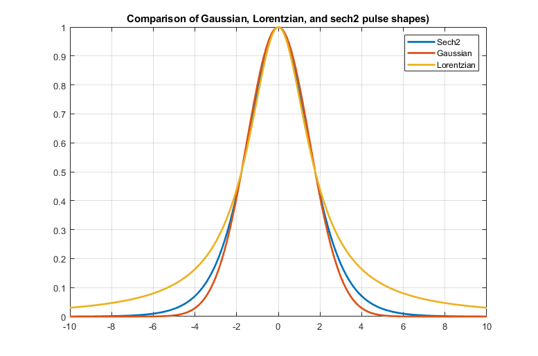
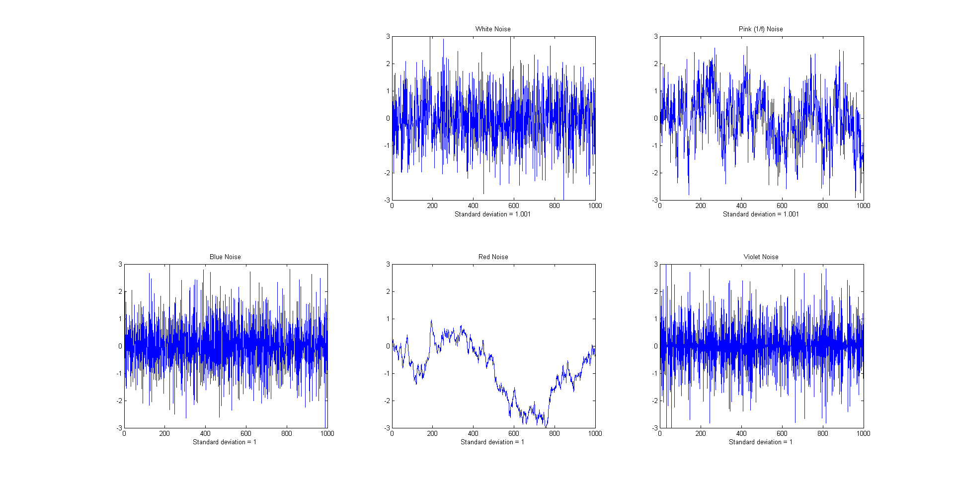
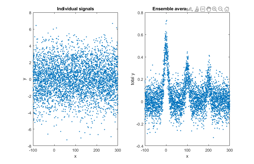
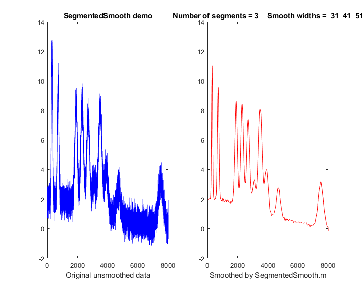
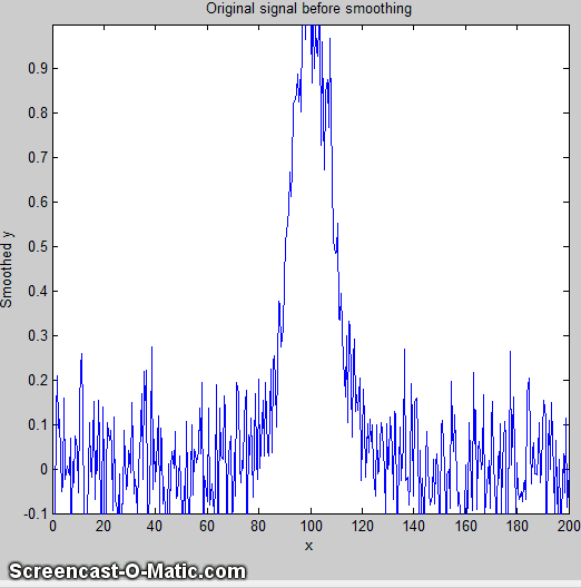
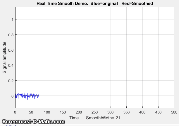
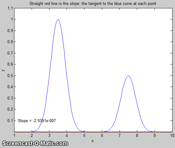
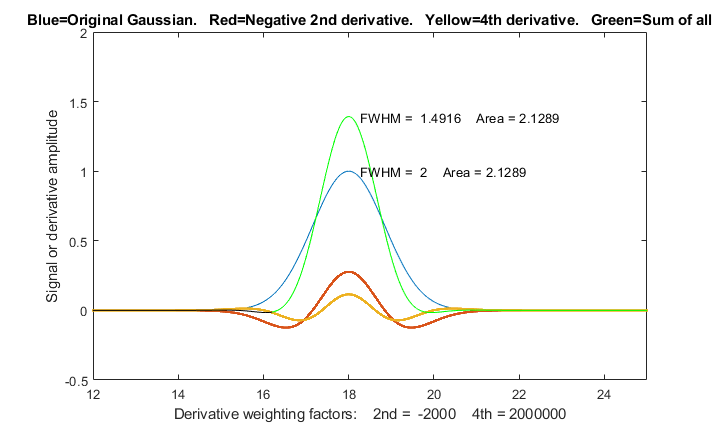
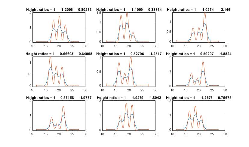
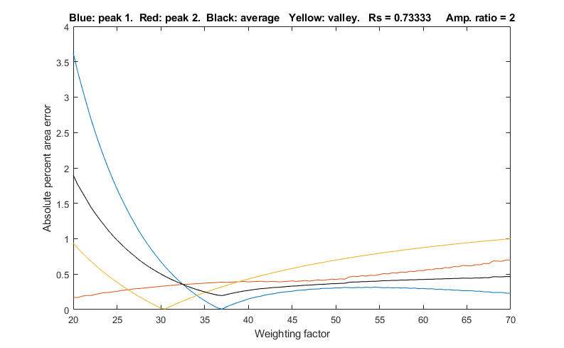
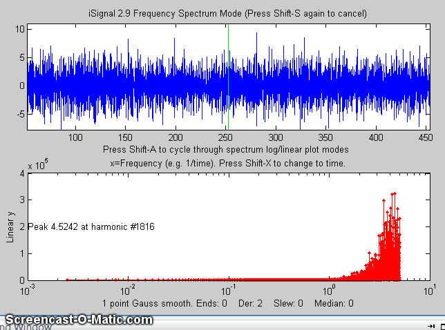
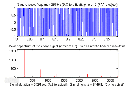
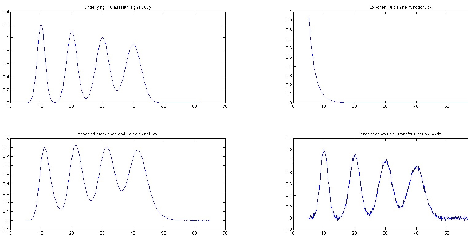
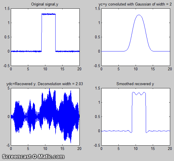
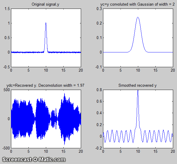
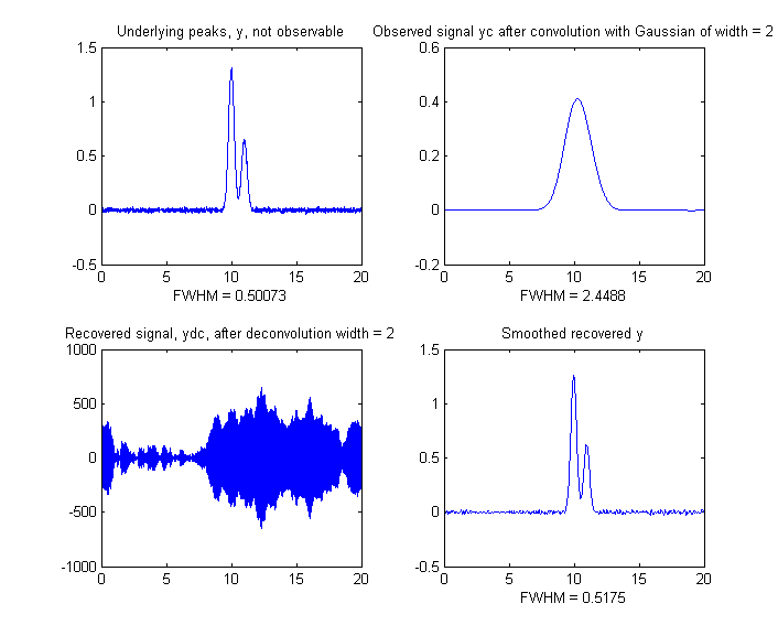
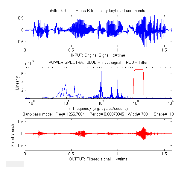
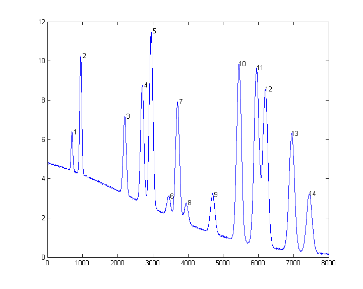
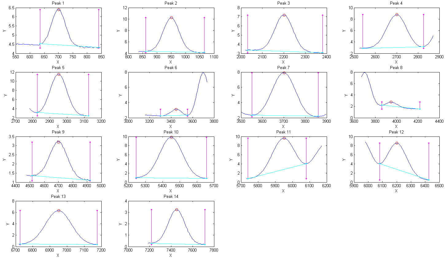
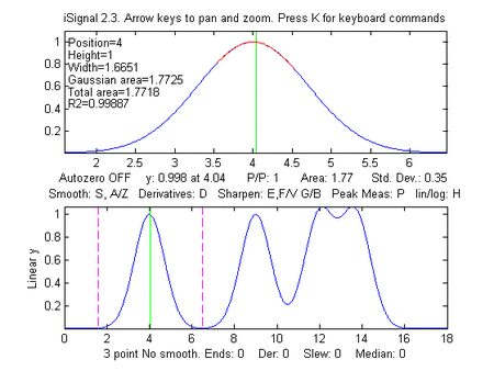
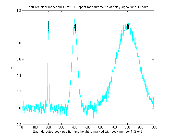
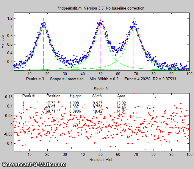
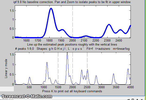
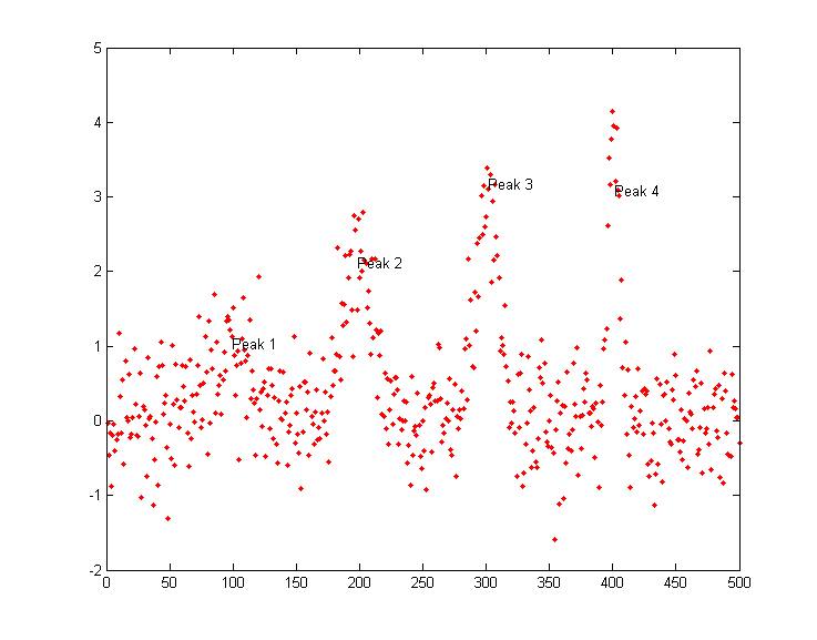
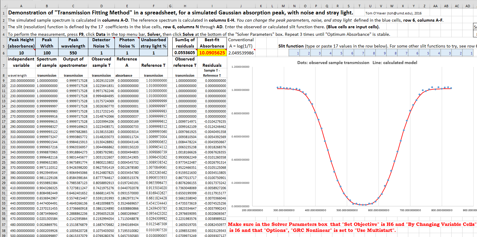