indexprevious next

Matlab/Octave Peak Fitters

[Peakfit.m]  [Peak shapes]  [Peakfit examples]  [Working with the FitResults matrix]  [Peakfit demos]  [Dealing with complex signals with lots of peaks[findpeaksfit]  [Interactive Peak Fitter (ipf.m) for Matlab]  [Animated instructions]  [ipf demos]  [Real data examples]  [ipf instructions]  [Hints and Tips]  [Live Script]  [Execution time]  [Extracting the equations for the best-fit models] [Adding a new peak shape]  [Have a question? Email me]

A Matlab peak fitting program for time-series signals, which uses an unconstrained non-linear optimization algorithm to decompose a complex, overlapping-peak signal into its component parts. The objective is to determine whether your signal can be represented as the sum of fundamental underlying peaks shapes. Accepts signals of any length, including those with non-integer and non-uniform x-values. There are two different versions,
(1) a command line version (peakfit.m) for Matlab or Octave, Matlab File Exchange "Pick of the Week". The current version number is 9.9, July 2021.
(2) a keypress operated interactive version ipf.m, or its Octave version ipfoctave. The current version number is 13.5.
The difference between them is that peakfit.m is completely controlled by command-line input arguments and returns its information via command-line output arguments; ipf.m allows interactive control via keypress commands. For automating the fitting of large numbers of signals, peakfit.m is better (see Appendix X for an example); but ipf.m is best for exploring signals to determine the optimum fitting range, peak shapes, number of peaks, baseline correction mode, etc. Otherwise they have similar curve-fitting capabilities. The basic built-in peak shape models available are illustrated in this graphic; custom peak shapes can be added. See Notes and Hints for more information and useful suggestions.

1. Matlab/Octave command-line function: peakfit.m (Version 9.9, July 2021)  

Peakfit.m is a user-defined command window peak fitting function for Matlab or Octave, usable from a remote terminal. It is written as a self-contained function in a single m-file. (To view of download, click peakfit.m). It takes data in the form of a 2 x n matrix that has the independent variables (X-values) in row 1 and the dependent variables (Y-values) in row 2, or as a single dependent variable vector. The syntax is [FitResults, GOF, baseline, coeff, residuals, xi, yi, BootResults] = peakfit(signal, center, window, NumPeaks, peakshape, extra, NumTrials, start, BaselineMode, fixedparameters, plots, bipolar, minwidth, DELTA, clipheight)). Only the first input argument, the data matrix, is absolutely required; there are default values for all other inputs. All the input and output arguments are explained below.
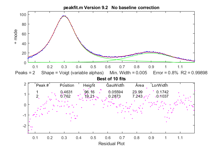
The screen display is shown on the right; the upper panel shows the data as blue dots, the combined model as a red line (ideally overlapping the blue dots), and the model components as green lines. The dotted magenta lines are the first-guess peak positions for the last fit. The lower panel shows the residuals (difference between the data and the model).

You can download a ZIP file containing peakfit.m, DemoPeakFit.m, ipf.m, Demoipf.m, some sample data for testing, and a test script (testpeakfit.m or autotestpeakfit.m) that runs all the examples sequentially to test for proper operation. For a discussion of the accuracy and precision of peak parameter measurement using peakfit.m, click here.

The peakfit.m functionality can also be accessed by the keypress-operated interactive functions ipf.m, iPeak.m, and iSignal.m. all of which contain peakfit.m as a sub-function.

Latest version 9.9: July 13, 2021, Fixed bug in Voigt (shapes 20 and 30) and added missing function for Gompertz, shape 43.

Peakfit.m can be called with several optional additional command line arguments. All input arguments (except the signal itself) can be replaced by zeros to use their default values.

peakfit(signal);     
  Performs an iterative least-squares fit of a single unconstrained Gaussian peak to the entire data matrix "signal", which has x values in row 1 and Y values in row 2 (e.g. [x y]) or which may be a single signal vector (in which case the data points are plotted against their index numbers on the x axis).
 
peakfit(signal,center,window);       
  Fits a single unconstrained Gaussian peak to a portion of the matrix "signal". The portion is centered on the x-value "center" and has width "window" (in x units). 

In this and in all following examples, set "center" and "window" both to 0 to fit the entire signal. 

peakfit(signal,center,window,NumPeaks);
  "NumPeaks" = number of peaks in the model (default is 1 if not specified).
 
peakfit(signal,center,window,NumPeaks,peakshape);
Number or vector that specifies the peak shape(s) of the model:  1=unconstrained Gaussian, 2=unconstrained Lorentzian, 3=logistic distribution, 4=Pearson, 5=exponentially broadened Gaussian; 6=equal-width Gaussians, 7=equal-width Lorentzians, 8=exponentially broadened equal-width Gaussians, 9=exponential pulse, 10= up-sigmoid (logistic function), 11=fixed-width Gaussians, 12=fixed-width Lorentzians13=Gaussian/Lorentzian blend; 14=bifurcated Gaussian, 15=Breit-Wigner-Fano resonance; 16=Fixed-position Gaussians; 17=Fixed-position Lorentzians; 18=exponentially broadened Lorentzian; 19=alpha function; 20=Voigt profile; 21=triangular; 23=down-sigmoid; 25=lognormal distribution; 26=linear baseline (see Example 28); 28=polynomial (extra=polynomial order; Example 30); 29=articulated linear segmented (see Example 29);  30=independently-variable alpha Voigt ; 31=independently-variable time constant ExpGaussian; 32=independently-variable Pearson; 33=independently-variable Gaussian/Lorentzian blend;  34=fixed-width Voigt; 35=fixed-width Gaussian/Lorentzian blend; 36=fixed-width exponentially-broadened Gaussian; 37=fixed-width Pearson; 38= independently-variable time constant ExpLorentzian; 39= alternative independently-variable time constant ExpGaussian (see Example 39 below); 40=sine wave;  41=rectangle; 42=flattened Gaussian; 43=Gompertz function (3 parameter logistic: Bo*exp(-exp((Kh*exp(1)/Bo)*(L-t)+1))); 44=1-exp(-k*x);  45: Four-parameter logistic y = maxy*(1+(miny-1)/(1+(x/ip)^slope)); 46=quadratic baseline (see Example 38); 47=blackbody emission; 48=equal-width exponential pulse; 49=Pearson IV (4 varibles); 50=multilinear regression (known peak positions and widths).

The function ShapeDemo demonstrates most of the basic peak shapes graphically, showing the variable-shape peaks as multiple lines.

Note 1: "unconstrained" simply means that the position, height, and width of each peak in the model can vary independently of the other peaks, as opposed to the equal-width, fixed-width, or fixed position variants. Shapes 4, 5, 13, 14, 15, 18, 20, and 34-37 are are constrained to the same shape constant; shapes 30-33 are completely unconstrained in position, width and shape; their shape variables are determined by iteration.
Note 2: The value of the shape constant "extra" defaults to 1 if not specified in input arguments.
Note 3: The peakshape argument can be a vector of different shapes for each peak, e.g. [1 2 1] for three peaks in a Gaussian, Lorentzian, Gaussian sequence. (The next input argument, 'extra', must be a vector of the same length as 'peakshape'. See Examples 24, 25, 28 and 38, below.

peakfit(signal,center,window,NumPeaks,peakshape,extra)
  Specifies the value of 'extra', used in the Pearson, exponentially-broadened Gaussian, Gaussian/Lorentzian blend, bifurcated Gaussian, and Breit-Wigner-Fano shapes to fine-tune the peak shape. The value of "extra" defaults to 1 if not specified in input arguments. In version 5, 'extra' can be a vector of different extra values for each peak).
  
peakfit(signal,center,window,NumPeaks,peakshape, extra, NumTrials);
  Restarts the fitting process "NumTrials" times with slightly different start values and selects the best one (with lowest fitting error). NumTrials can be any positive integer (default is 1). In may cases, NumTrials=1 will be sufficient, but if that does not give consistent results, increase NumTrials until the result are stable. 
 
peakfit(signal,center,window,NumPeaks,peakshape,extra, NumTrials, start)
  Specifies the first guesses vector "firstguess" for the peak positions and widths, e.g. start=[position1 width1 position2 width2 ...].  Only necessary on difficult cases, especially when there are a lot of adjustable variables. The start vector can be the approximate average values based on your experience, or it can be calculated from a previous simpler fit, as in this example.  If you leave this off, or set start=0, the program will generate its own start values (which is often good enough).

peakfit(signal,center,window,NumPeaks,peakshape,extra, NumTrials, start, BaselineMode)
As above, but "BaselineMode" sets the baseline correction mode in the last argument:
BaselineMode=0 (default) does not subtract baseline from data segment;. BaselineMode=1 interpolates a linear baseline from the edges of the data segment and subtracts it from the signal (assumes that the peak returns to the baseline at the edges of the signal); BaselineMode=2,  like mode 1 except that it computes a quadratic curved baseline; BaselineMode=3 compensates for a flat baseline without reference to the signal itself (does not require that the signal return to the baseline at the edges of the signal, as does modes 1 and 2). Coefficients of the polynomial baselines are returned in the third output argument "baseline".

peakfit(signal,0,0,0,0,0,0,0,2)
  Use zeros as placeholders to use the default values of input arguments.  In this case,
BaselineMode is set to 2, but all others are the default values.

peakfit(signal,center,window,NumPeaks,peakshape, extra, NumTrials, start, BaselineMode, fixedparameters)
 'fixedparameters' (10th input argument) specifies fixed widths or positions in shapes 11, 12, 16, 17, 34-37, one entry for each peak When using peak shape 50 (multlinear regression), 'fixedparameters' must be a matrix listing the peak shape number (column 1), position (column 2), and width (column 3) of each peak, one row per peak. 
 
peakfit(signal,center,window,NumPeaks,peakshape,extra, NumTrials, start, BaselineMode, fixedparameters, plots)
 'plots' (11th input argument) controls graphic plotting: 0=no plot; 1=plots draw as usual (default)
 
peakfit(signal,center,window,NumPeaks,peakshape,extra,NumTrials, start, BaselineMode, fixedparameters, plots, bipolar)
 (12th input argument) 'bipolar' = 0 constrain peaks heights to be positive; 'bipolar' = 1 allows positive and negative peak heights.
 
peakfit(signal,center,window,NumPeaks,peakshape,extra,NumTrials, start, BaselineMode, fixedparameters, plots, bipolar, minwidth)
  'minwidth' (13th input argument) sets the minimum allowed peak width. The default if not specified is equal to the x-axis interval. Must be a vector of minimum  widths, one value for each peak, if the multiple peak shape is chosen.

peakfit(signal,center,window,NumPeaks,peakshape,extra, NumTrials, start, BaselineMode, fixedparameters, plots, bipolar, minwidth, DELTA)
 'DELTA' (14th input argument) controls the restart variance when NumTrials>1. Default value is 1.0. Larger values give more variance. Version 5.8 and later only.

[FitResults,FitError]= peakfit(signal,center,window...);
Returns the FitResults vector in the order peak number, peak position, peak height, peak width, and peak area), and the FitError (the percent RMS difference between the data and the model in the selected segment of that data) of the best fit.

Labeling the FitResults table: Using the "table" function, you can display FitResults in a neat table with column labels in a single line of code:
disp(table(FitResults(:,2), FitResults(:,3), FitResults(:,4), FitResults(:,5), 'VariableNames', {'Position' 'Height' 'FWHM' 'Area'}))

Position      Height       FWHM        Area      
________    ________      ______    __________  
8.0763      3.8474        10.729    3.4038e-01  
  20           1              3        3.1934  
  

Additional columns of FitResults and VariableNames can be added for those peak shapes that display five or more results, such as the voigt shape:
disp(table(FitResults(:,2), FitResults(:,3), FitResults(:,4), FitResults(:,5), FitResults(:,6), 'VariableNames', {'Position' 'Height' 'GauWidth' 'Area' 'LorWidth'}))


Position  Height  GauWidth   Area    LorWidth
________  _______  ________  _______   ________
0.80012  0.99987  0.30272   0.34744   0.39708
1.2003   0.79806  0.40279   0.27601   0.30012


Calculating the precision of the peak parameters:
[FitResults, GOF, baseline, coeff, residuals, xi, yi, BootstrapErrors] = peakfit([x;y],0,0,2,6,0,1,0,0,0);

Displays parameter error estimates by the bootstrap method; See DemoPeakfitBootstrap for a self-contained demo of this function.

Optional output parameters:
  1.   FitResults: a table of model peak parameters, one row for each peak, listing peak number, peak position, height, width, and area (or, for shape 28, the polynomial coefficients, and for shape 29, the x-axis breakpoints).
  2.  GOF ("Goodness of Fit"), a 2-element vector containing the RMS fitting error of the best trial fit and the R-squared (coefficient of determination).
  3.   baseline: returns the polynomial coefficients of  the interpolated baseline in linear and quadratic baseline modes (1 and 2) or the value of the constant baseline in flat baseline mode.
  4.   coeff: Coefficients for the polynomial fit (shape 28 only; for other shapes, coeff=0)
  5.   residual: vector of differences between the data and the best fit model. Can be used to measure the characteristics of the noise in the signal.
  6.   xi: vector containing 600 interpolated x-values for the model peaks.
  7.   yi: matrix containing the y values of model peaks at each xi. Type plot(xi,yi(1,:)) to plot peak 1 or plot(xi,yi) to plot all the peaks
  8.   BootstrapErrors: a matrix containing bootstrap standard deviations and interquartile ranges for each peak parameter of each peak in the fit.


Examples:
Note: test script testpeakfit.m runs all the following examples automatically; just press Enter to continue to the next one. (You can copy and paste, or drag and drop, any of these single-line or multi-line code examples into the Matlab or Octave editor or into the command line and press Enter to execute it).

Example 1.  Fits computed x vs y data with a single unconstrained Gaussian peak model.
  > x=[0:.1:10];y=exp(-(x-5).^2); peakfit([x' y'])
  ans = 
Peak Position Height  Width  Peak area

1       5        1    1.665   1.7725

Example 2. Fits small set of manually-entered y data to a single unconstrained Gaussian peak model.  
  > y=[0 1 2 4 6 7 6 4 2 1 0 ]; x=1:length(y);
  > peakfit([x;y],length(y)/2,length(y),0,0,0,0,0,0)

Peak  Position   Height  Width   Peak area
  1    6.0001    6.9164  4.5213    32.98


Example 3.  Measurement of very noisy peak with signal-to-noise ratio = 1. (Try several times).
> x=[0:.01:10];y=exp(-(x-5).^2) + randn(size(x)); peakfit([x;y])
 
Peak   position  Height   Width   Peak area
   1   5.0951  1.0699  1.6668  1.8984

Example 4.  
Fits a noisy two-peak signal with a two-peak unconstrained Gaussian model (NumPeaks=2).
  > x=[0:.1:10]; y=exp(-(x-5).^2)+.5*exp(-(x-3).^2) + .1*randn(1,length(x));
 > peakf([x' y'],5,19,2,1,0,1)
Peak        Position   Height   Width   Peak area
   1       3.0001    0.49489   1.642   0.86504
   2       4.9927    1.0016    1.6597  1.7696

Example 5.
Fits a portion of the humps function, 0.7 units wide and centered on x=0.3, with a single (NumPeaks=1) Pearson function (peakshape=4) with extra=3 (controls shape of Pearson function).
    > x=[0:.005:1];y=humps(x);peakfit([x' y'],.3,.7,1,4,3);
    
Example 6. Creates a data matrix 'smatrix', fits a portion to a two-peak unconstrained Gaussian model, takes the best of 10 trials.  Returns optional output arguments FitResults and FitError.
  > x=[0:.005:1]; y=(humps(x)+humps(x-.13)).^3; smatrix=[x' y'];
 > [FitResults,FitError]=peakfit(smatrix,.4,.7,2,1,0,10)
Peak Position   Height      Width      Peak area
1     0.4128  3.1114e+008   0.10448   3.4605e+007
2     0.3161  2.8671e+008   0.098862  3.0174e+007
   FitError = 0.68048
 
Example 7. As above, but specifies the first-guess position and width of the two peaks, in the order [position1 width1 position2 width2]
  > peakfit([x' y'],.4,.7,2,1,0,10,[.3 .1 .5 .1]);

Supplying a first guess
position and width is also useful if you have one peak on top of another (like example 4, with both peaks at the same position x=5, but with different widths):
>> x=[2:.01:8];y=exp(-((x-5)/.2).^2)+.5.*exp(-(x-5).^2)+.1*randn(1,length(x));
>> peakfit([x' y'],0,0,2,1,0,1,[5 2 5 1])

Peak Position   Height     Width      Peak area
  1    4.9977   0.51229    1.639      0.89377
  2    4.9948   1.0017   0.32878      0.35059

Example 8. As above, returns the vector xi containing 600 interpolated x-values for the model peaks and the matrix yi containing the y values of each model peak at each xi.  Type plot(xi,yi(1,:)) to plot peak 1 or  plot(xi,yi,xi,sum(yi)) to plot all the model components and the total model (sum of components).
> [FitResults, GOF, baseline, coeff, residuals,xi,yi]= peakfit(smatrix,.4,.7,2,1,0,10);
> figure(2):clf;
plot(xi,yi,xi,sum(yi))

Example 9. Fitting a single unconstrained Gaussian on a linear background, using the linear BaselineMode mode (9th input argument = 1)
    >>x=[0:.1:10]';y=10-x+exp(-(x-5).^2);peakfit([x y],5,8,0,0,0,0,0,1)

Example 10. Fits a group of three peaks near x=2400 in DataMatrix3 with three equal-width exponentially-broadened Gaussians.

>> load DataMatrix3
>> [FitResults,FitError]= peakfit(DataMatrix3,2400,440,3,8,31,1)

Peak     Position   Height     Width    Peak area
  1       2300.5     0.82546   60.535    53.188
  2       2400.4     0.48312   60.535    31.131
  3       2500.6     0.84799   60.535    54.635
FitError = 0.19975

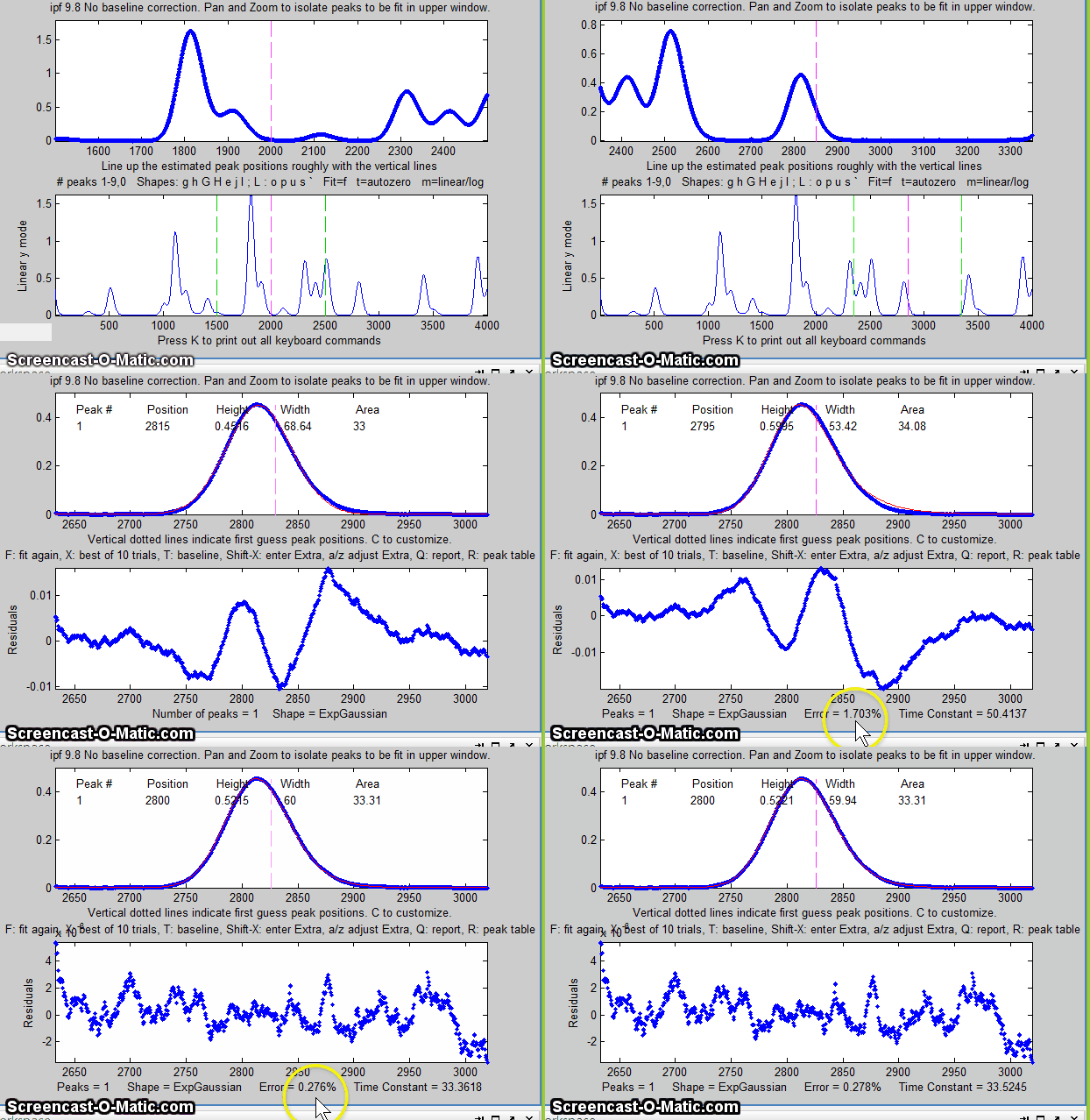
Note: if your peaks are trailing off to the left, rather that to the right as in the above example, simply use a negative value for the time constant (in ipf.n, press Shift-X and type a negative value).

Example 11.  Example of an unstable fit to a signal consisting of two unconstrained Gaussian peaks of equal height (1.0). The peaks are too highly overlapped for a stable fit, even though the fit error is small and the residuals are unstructured. Each time you re-generate this signal, it gives a different fit, with the peaks heights varying about 15% from signal to signal.  
>> x=[0:.1:10]'; y=exp(-(x-5.5).^2) + exp(-(x-4.5).^2) + .01*randn(size(x)); [FitResults,FitError]= peakfit([x y],5,19,2,1)

Peak  Position   Height    Width   Peak area
1       4.4059   0.80119   1.6347   1.3941
2       5.3931    1.1606   1.7697   2.1864
FitError = 0.598

  Much more stable results can be obtained using the equal-width Gaussian model (
peakfit([x y],5,19,2,6)), but that is justified only if the experiment is legitimately expected to yield peaks of equal width. See http://terpconnect.umd.edu/~toh/spectrum/CurveFittingC.html#Peak_width_constraints.

Example 12.  Baseline correction. Demonstration of the four BaselineMode modes, for a single Gaussian on large baseline, with position=10, height=1, and width=1.66. The BaselineMode mode is specified by the 9th input argument (0,1,2, or 3).

BaselineMode=0 means to ignore the baseline (default mode if not specified). In this case, this leads to large errors.
>>
x=8:.05:12;y=1+exp(-(x-10).^2);
>> [FitResults,FitError,baseline]=peakfit([x;y],0,0,1,1,0,1,0,0)
  FitResults =
     1     10    1.8561     3.612  5.7641
 FitError =5.387
 baseline = 0

BaselineMode=1 subtracts linear baseline from edge to edge. Does not work well in this case because the signal does not return completely to the baseline at the edges.
>> [FitResults,FitError,baseline]=peakfit([x;y],0,0,1,1,0,1,0,1)
FitResults =
    1    9.9984   0.96161  1.5586  1.5914
FitError = 1.9801
baseline = 0.0012608     1.0376

  BaselineMode=2 subtracts quadratic baseline from edge to edge. Does not work well in this case because the signal does not return
completely to the baseline at the edges.
>> [FitResults,FitError,baseline]=peakfit([x;y],0,0,1,1,0,1,0,2)
FitResults =
1    9.9996  0.81762    .4379   1.2501
FitError = 1.8205
baseline = -0.046619     0.9327     -3.469

BaselineMode=3 subtracts a flat baseline automatically, without requiring that the signal returns to baseline at the edges. This mode works best for this signal.
>> [FitResults,FitError,baseline]=peakfit([x;y],0,0,1,1,0,1,0,3)

FitResults =
1        10    1.0001    1.6653    1.7645
FitError = 0.0037056
baseline = 0.99985

In the following example, the baseline is strongly sloped, but straight. In that case the most accurate result is obtained by using a 2-peak fit, fitting the baseline with a variable-slope straight line (shape 26, peakfit version 6 only).
>> x=8:.05:12;y=x+exp(-(x-10).^2);
>>
[FitResults,FitError]=peakfit([x;y],0,0,2,[1 26],[1 1],1,0)
FitResults =           
1      10      1     1.6651   1.7642
2      4.485  0.223  0.05   40.045
FitError =0.093

In this example, the baseline is curved, so you may be able to get good results with BaselineMode=2:
>> x=[0:.1:10]';y=1./(1+x.^2)+exp(-(x-5).^2);
>> [FitResults,FitError,baseline]=peakfit([x y],5,5.5,0,0,0,0,0,2)
FitResults =
1     5.0091    0.97108     1.603    1.6569
FitError = 0.97661
baseline = 0.0014928    -0.038196      0.22735

Example 13. Same as example 4, but with fixed-width Gaussian (shape 11), width=1.666. The 10th input argument is a vector of fixed peak widths, one entry for each peak, which may be the same or different for each peak.
>> x=[0:.1:10];y=exp(-(x-5).^2)+.5*exp(-(x-3).^2)+.1*randn(size(x));
>> [FitResults,FitError]=peakfit([x' y'],0,0,2,11,0,0,0,0,[1.666 1.666])

         Peak    Position   Height     Width   Peak area
           1      3.9943    0.49537     1.666   0.87849
           2      5.9924    0.98612     1.666    1.7488

Example 14. Peak area measurements. Same as the example in Figure 15 on Integration and Peak Area Measurement.  All four peaks have the same theoretical peak area (1.772). The four peaks can be fit together in one fitting operation using a 4-peak Gaussian model, with only rough estimates of the first-guess positions and widths.  The peak areas thus measured are much more accurate than the perpendicular drop method:
>> x=[0:.01:18];
>> y=exp(-(x-4).^2)+exp(-(x-9).^2)+exp(-(x-12).^2)+exp(-(x-13.7).^2);
>> peakfit([x;y],0,0,4,1,0,1,[4 2 9 2 12 2 14 2],0,0)

         Peak    Position   Height   Width    Peak area
           1            4      1     1.6651    1.7725
           2            9      1     1.6651    1.7725
           3           12      1     1.6651    1.7724
           4         13.7      1     1.6651    1.7725

This works well even in the presence of substantial amounts of random noise:
>> x=[0:.01:18]; y=exp(-(x-4).^2)+exp(-(x-9).^2)+exp(-(x-12).^2)+exp(-(x-13.7).^2)+.1.*randn(size(x));
>> peakfit([x;y],0,0,4,1,0,1,[4 2 9 2 12 2 14 2],0,0)

Peak  Position   Height    Width    Peak area
  1    4.0086   0.98555   1.6693    1.7513
  2    9.0223    1.0007   1.669     1.7779
  3    11.997    1.0035   1.6556    1.7685
  4    13.701    1.0002   1.6505    1.7573

Sometimes experimental peaks are effected by exponential broadening, which does not by itself change the true peak areas, but does shift peak positions and increases peak width, overlap, and asymmetry, as shown when you try to fit the peaks with Gaussians. Using the same noise signal from above:
>> y1=ExpBroaden(y',-50);
>> peakfit([x;y1'],0,0,4,1,50,1,0,0,0)

Peak number  Position  Height Width   Peak area

     1       4.4538  0.83851  1.9744  1.7623
     2       9.4291  0.8511   1.9084  1.7289
     3       12.089  0.59632  1.542   0.97883
     4       13.787   1.0181  2.4016  2.6026

Peakfit.m (and ipf.m) have an exponentially-broadened Gaussian peak shape (shape #5) that works better in those cases:, recovering the original peak positions, heights, widths, and areas. (Adding a first-guess vector as the 8th argument may improve the reliability of the fit in some cases).
>> y1=ExpBroaden(y',-50);
>> peakfit([x;y1'],0,0,4,5,50,1,[4 2 9 2 12 2 14 2],0,0)
Peak#    Position      Height    Width       Area
1            4           1       1.6651     1.7725
2            9           1       1.6651     1.7725
3           12           1       1.6651     1.7725
4         13.7     0.99999       1.6651     1.7716

An easy way to obtain a good first-guess vector for an exponentially broadened Gaussian fit is to perform a simple Gaussian fit initially and have the script use the FitResults matrix from that fit, plus an estimate of the time constant, to construct the first-guess vector, as in this example.

Example 15. Displays a table of parameter error estimates. See DemoPeakfitBootstrap for a self-contained demo of this function.
>> x=0:.05:9; y=exp(-(x-5).^2)+.5*exp(-(x-3).^2)+.01*randn(1,length(x));
>> [FitResults,LowestError,baseline,residuals,xi,yi,BootstrapErrors]= peakfit([x;y],0,0,2,6,0,1,0,0,0);

Peak #1       Position    Height       Width       Area
Mean:        2.9987      0.49717     1.6657      0.88151
STD:         0.0039508   0.0018756   0.0026267   0.0032657
STD (IQR):   0.0054789   0.0027461   0.0032485   0.0044656
% RSD:       0.13175     0.37726     0.15769     0.37047
%
RSD {IQR): 0.13271     0.35234     0.16502     0.35658
 
Peak #2       Position    Height       Width       Area
Mean:        4.9997     0.99466       1.6657      1.7636
STD:         0.001561   0.0014858     0.00262     0.0025372
STD (IQR):   0.002143   0.0023511     0.00324     0.0035296
% RSD:       0.031241   0.14938       0.15769     0.14387
%
STD (IQR): 0.032875   0.13637       0.16502     0.15014

Example 16. Fits both peaks of the Humps function with a Gaussian/Lorentzian blend (shape 13) that is 15% Gaussian (Extra=15). The 'Extra' argument sets the percentage of Gaussian shape.
>> x=[0:.005:1];y=humps(x);[FitResults,FitError]= peakfit([x' y'],0.54,0.93,2,13,15,10,0,0,0)
 FitResults =
     1     0.30078      190.41     0.19131      23.064
     2     0.89788      39.552     0.33448      6.1999
  FitError = 0.34502

Example 17. 
Fit a slightly asymmetrical peak with a bifurcated Gaussian (shape 14). The 'Extra' argument (=45) controls the peak asymmetry (50 is symmetrical). 
>> x=[0:.1:10];y=exp(-(x-4).^2)+.5*exp(-(x-5).^2)+.01*randn(size(x));

>> [FitResults,FitError]=peakfit([x' y'],0,0,1,14,45,10,0,0,0)
 FitResults =
     1     4.2028     1.2315      4.077     2.6723
  FitError =0.84461

Example 18.
Returns output arguments only, without plotting or command window printing (11th input argument = 0, default is 1)
>> x=[0:.1:10]';y=exp(-(x-5).^2);FitResults=peakfit([x y],0,0,1,1,0,0,0,0,0,
0)

Example 19.  Same as example 4, but with fixed-position Gaussian (shape 16), positions=[3 5]
>> x=[0:.1:10];y=exp(-(x-5).^2)+.5*exp(-(x-3).^2)+.1*randn(size(x));
>> [FitResults,FitError]=peakfit([x' y'],0,0,2,16,0,0,0,0,[3 5])

    Peak  Position   Height        Width      Peak area
      1       3      0.49153       1.6492      0.86285
      2       5       1.0114       1.6589        1.786
FitError =8.2693

Example 20.  Exponentially modified Lorentzian (shape 18) with added noise. As for peak shape 5, peakfit.m recovers the original peak position (9), height (1), and width (1).

>> x=[0:.01:20]; L=lorentzian(x,9,1)+0.02.*randn(size(x));
L1=ExpBroaden(L',-100);
>> peakfit([x;L1'],0,0,1,18,100,1,0,0)

Example 21. Fitting humps function with two unconstrained Voigt profiles  (version 9.2)
>> disp('Peak #  Position  Height  GauWidth   Area  LorWidth')
>> [FitResults,FitError]=peakfit(humps(0:.01:2),60,120,2,30,1.7,5,0)
FitResults =
    1   48.555    95.09   7.1121   2413.8   16.485
    2   78.173   19.602   20.377   769.04   19.775

GOF =
      0.72829      0.9991
5

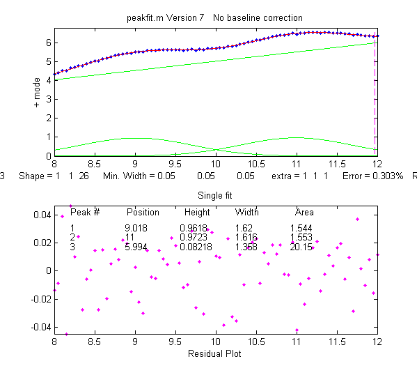
Example 22. peakfitdemob.m. Illustrated on the right. Measurement of three weak Gaussian peaks at x=100, 250, 400, superimposed in a very strong curved baseline plus noise. The peakfit function fits four peaks, treating the baseline as a 4th peak whose peak position is negative. Because this results in so many adjustable variables (4 peaks x 2 variable/peak = 8 variables), you need to specify a "start" vector, like Example 7. You can test the reliability of this method by changing the peak parameters in lines 11, 12, and 13 and see if the peakfit function will successfully track the changes and give accurate results for the three peaks without having to change the start vector. See Example 9 on iSignal.html for other ways to handle this signal. (The true peaks heights are 1, 2, and 3, respectively).
Example 23. 12th input argument (+/- mode) set to 1 (bipolar) to allow negative as well as positive peak heights. (Default is 0)
  >> x=[0:.1:10];y=exp(-(x-5).^2)-.5*exp(-(x-3).^2)+.1*randn(size(x));
  >> peakfit([x' y'],0,0,2,1,0,1,0,0,0,1,1)
  FitResults =
       1    3.1636   -0.5433      1.62   -0.9369
       2    4.9487   0.96859    1.8456    1.9029
  FitError =8.2757

Example 24. Version 5 or later. Fits humps function to a model consisting of one Lorentzian and one Gaussian peak.
   
>> x=[0:.005:1.2];y=humps(x);[FitResults,FitError]=peakfit([x' y'],0,0,2,[2 1],[0 0])
  FitResults =
      1    0.30178    97.402   0.18862    25.116
      2    0.89615    18.787   0.33676    6.6213
  FitError = 1.0744

 
Example 25. Version 5 or later: Five peaks,
five different shapes, all heights = 1, all widths = 3, "extra" vector included for peaks 4 and 5.
  x=0:.1:60;
  y=modelpeaks2(x,[1 2 3 4 5],[1 1 1 1 1],[10 20 30 40 50],[3 3 3 3 3],[0 0 0 2 -20])+.01*randn(size(x));
  peakfit([x' y'],0,0,5,[1 2 3 4 5],[0 0 0 2 -20])  

You can also use this technique to create models with all the same shapes but with different values of  'extra' using a vector of 'extra' values, or (in version 5.7) with different minimum width restrictions by using a vector of  'minwidth' values as input argument 13.

Example 26.
Version 5.7 or later: Minimum width constraint (13th input argument)
  >> x=1:30;y=gaussian(x,15,8)+.05*randn(size(x));
  No constraint (minwidth=0):
  peakfit([x;y],0,0,5,1,0,10,0,0,0,1,0,0);
  Widths constrained to values 7 or above:
  peakfit([x;y],0,0,5,1,0,10,0,0,0,1,0,7);

Example 27. Noise test with very noisy peak signal: peak height = RMS noise = 1.
    >> x=[-10:.05:10];y=exp(-(x).^2)+randn(size(x));P=peakfit([x;y],0,0,1,1,0,10);

Example 28: Weak Gaussian peak on sloped straight-line baseline, 2-peak fit with one Gaussian and one variable-slope straight line ('slope', shape 26, peakfit version 6 only).
  >> x=8:.05:12;y=x+exp(-(x-10).^2); [FitResults,FitError]= peakfit([x;y],0,0,2,[1 26],[1 1],1,0)
  FitResults =          
       1      10    1     1.6651  1.7642
       2   4.485  0.223   0.05    40.045
  FitError =0.093
  As above, with two overlapping signal peaks, using a 3-peak fit with peakshape=[1 1 26], helped by adding rough first guesses ('start') using the 'polyfit' function to generate automatic first guesses for the sloping baseline. The third component (peak 3) is the baseline.
x=8:.05:12
y=x/2+exp(-(x-9).^2)+exp(-(x-11).^2)+.02.*randn(size(x));

start=[8 1 10 1 polyfit(x,y,1)];
[FitResults,FitError]=peakfit([x;y],0,0,3,[1 1 26],[1 1 1],1,start)
 See example 38 for a similar example with a curved baseline. Screen image on the right -->.

 
Example 29: Segmented linear fit (Shape 29, peakfit version 6 only). You specify the number of segments in the 4th input argument ('NumPoints') and the program attempts to find the optimum x-axis positions of the breakpoints that minimize the fitting error. The vertical dashed magenta lines mark the x-axis breakpoints. Another example with a single Gaussian band .
  >> x=[0.9:.005:1.7];y=humps(x);
  >> peakfit([x' y'],0,0,9,29,0,10,0,0,0,1,1)
 
 Example 30: Polynomial fit (Shape 28, peakfit version 6 only). Specify the order of the polynomial (any positive integer) in the 6th input argument ('extra'). (The 12th input argument, 'bipolar', is set to 1 to plot the entire y-axis range when y goes negative).

  >> x=[0.3:.005:1.7];y=humps(x);y=y+cumsum(y);
  >> peakfit([x' y'],0,0,1,28,6,10,0,0,0,1,1)

Example 31: The Matlab/Octave script NumPeaksTest.m uses peakfit.m to demonstrate one way to determine the minimum number of model peaks needed to fit a set of data, plotting the fitting error vs the number of model peaks, and looking for the point at which the fitting error reaches a minimum. This script creates a noisy computer-generated signal containing a user-selected 3, 4, 5 or 6 underlying peaks, fits to a series of models containing 1 to 10 model peaks, plots the fitting errors vs the number of model peaks and then determines the vertex of  the best-fit parabola; the nearest integer is usually the correct number of peaks underlying peaks. Also requires that the plotit.m function be installed.

Example 32: Version 7 and later supports unconstrained variable shapes 30-33 and 39 that have three iterated variables (position, width, and shape):
 a.  Voigt (shape 30). In version 9.2, this returns separate Gaussian and Lorentzian widths:
  x=1:.1:30; y=modelpeaks2(x,[13 13],[1 1],[10 20],[3 3],[20 80]);
  disp('Peak #  Position   Height   GauWidth  Area  LorWidth')
  [FitResults,FitError] = peakfit([x;y],0,0,2,30,2,10)
.
 b. Exponentially broadened Gaussian (shape 31): load DataMatrix3;
  [FitResults,FitError] = peakfit(DataMatrix3, 1860.5, 364, 2, 31, 32.9731, 5,[1810 60 30 1910 60 30])
    Version 8.4 also includes an alternative exponentially broadened Gaussian , shape 39, which is parameterized differently (see Example 39).
 c. Pearson (shape 32)  x=1:.1:30; y=modelpeaks2(x,[4 4],[1 1],[10 20],[5 5],[1 10]);
  [FitResults,FitError] = peakfit([x;y],0,0,2,32,0,5)

 d. Gaussian/Lorentzian blend (shape 33): x=1:.1:30; y=modelpeaks2(x,[13 13],[1 1],[10 20],[3 3],[20 80]);
  [FitResults,FitError]=peakfit([x;y],0,0,2,33,0,5)


Example 34:
Using the built-in "sortrows" function to sort the FitResults table by peak position (column 2) or peak height (column 3).
 >> x=[0:.005:1.2]; y=humps(x); [FitResults,FitError]=peakfit([x' y'],0,0,3,1)
 >> sortrows(FitResults,2)
ans =
   2    0.29898     56.463    0.14242     8.5601
   1    0.30935     39.216    0.36407     14.853
   3    0.88381     21.104    0.37227     8.1728
>> sortrows(FitResults,3)
ans =
   3    0.88381     21.104    0.37227     8.1728
   1    0.30935     39.216    0.36407     14.853
   2    0.29898     56.463    0.14242     8.5601

Example 35: Version 7.6 or later. Using the fixed-width Gaussian/Lorentzian blend (shape 35).

  >> x=0:.1:10; y=GL(x,4,3,50)+.5*GL(x,6,3,50) + .1*randn(size(x));
  >> [FitResults,FitError]=peakfit([x;y],0,0,2,35,50,1,0,0,[3 3])

   peak    position    height    width    area
    1      3.9527     1.0048       3     3.5138
    2      6.1007     0.5008       3     1.7502
  GoodnessOfFit
= 6.4783      0.95141

Compared to variable-width fit (shape 13),  the fitting error is larger but nevertheless results are more accurate (when true peak width is known, width = [3 3]).   
>> [FitResults,GoodnessOfFit]= peakfit([x;y],0,0,2,13,50,1)
     1     4.0632    1.0545     3.2182   3.9242
     2     6.2736    0.41234    2.8114   1.3585
  GoodnessOfFit
= 6.4311      0.95211

Note: to display the FitResults table with column labels, call peakfit.m with output arguments [FitResults...] and type :
 

disp('      Peak number  Position      Height      Width       Peak area');disp(FitResults)
Example 36: Variable time constant exponentially-broadened Lorentzian function, shape 38. (Version 7.7 and above only). FitResults has an added 6th column for the measured time constant.
  >> x=[1:100]';
  >> y=explorentzian(x',40,5,-10)+.01*randn(size(x));
  >> peakfit([x y],0,0,1,38,0,10)

Example 37: 3-parameter logistic (Gompertz), shape 43. (Version 7.9 and above only). Parameters labeled Bo, Kh, and L. FitResults extended to 6 columns.
>> t=0:.1:10;
>> Bo=6;Kh=3;L=4;
>> y=Bo*exp(-exp((Kh*exp(1)/Bo)*(L-t)+1))+.1.*randn(size(t));
>> [FitResults,GOF]=peakfit([t;y],0,0,1,43)

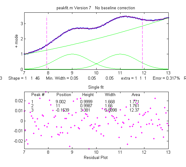
Example 38: Shape 46, 'quadslope' (version 8 and above). Two overlapping Gaussians (position=9,11; heights=1; widths=1.666) on a curved baseline, using a 3-peak fit with peakshape=[1 1 46], default NumTrials and start. Screen image on the right -->.
>> x=7:.05:13;
>> y=x.^2/50+exp(-(x-9).^2)+exp(-(x-11).^2)+.01.*randn(size(x));
>> [FitResults,FitError]=peakfit([x;y],0,0,3,[1 1 46],[1 1 1])
Note: if the baseline is much higher in amplitude that the peak amplitude, it will help to supply an approximate 'start' value and to use NumTrials > 1.

Example 39: Comparison of alternative unconstrained exponentially broadened Gaussians, shapes 31 and 39. Shape 31 (expgaussian.m) creates the shape by performing a Fourier convolution of a specified Gaussian by an exponential decay of specified time constant, whereas shape 39 (expgaussian2.m) uses a mathematical expression for the final shape so produced. Both result in the same peak shape but are parameterized differently. Shape 31 reports the peak height and position as that of the original Gaussian before broadening, whereas shape 39 reports the peak height of the broadened result. Shape 31 reports the width as the FWHM (full width at half maximum) and shape 39 reports the standard deviation (sigma) of the Gaussian. Shape 31 reports the exponential factor an the number of data points and shape 39 reports the reciprocal of time constant in time units. See the script GaussVsExpGauss.m (graphic); See Figure windows 2 and 3. For multiple-peak fits, both shapes usually require a reasonable first guess ('start") vector for best results.

Method  Position  Height Halfwidth  Area   Exp. factor
Shape 31  10        1        5      5.3223   20.0001
Shape 39  12.8282  0.35578  11.7731 5.3217    0.1
See the script DemoExpgaussian.m for a more detailed explanation.

Example 40: Use of the "start" vector in 4-Gaussian fit to the "humps" function.

  x=[-.1:.005:1.2];y=humps(x);

 First attempt with default start values gives poor fit:

 [FitResults,GOF]=peakfit([x;y],0,0,4,1,0,10)

 Second attempt specifying approximate start values in the 8th input argument gives almost perfect fit:

 start=[0.3 0.13 0.3 0.34 0.63 0.15 0.89 0.35];

 [FitResults,GOF]=peakfit([x;y],0,0,4,1,0,10,start)

Example 41: Peakfit 9 and above. Use of peak shape 50 ("multilinear regression") when the peak positions and widths are known, and only the peak heights are unknown. The peak shapes, positions, and widths are specified in the 10th input argument "fixedparameters", which must in this case be a matrix listing the peak shape number (column 1), position (column 2), and width (column 3) of each peak, one row per peak. See the demonstration scripts peakfit9demo.m and peakfit9demoL.m.

Example 42: RandPeaks.m is a script that demonstrates the accuracy of iterative peak fitting when no customized "start" values are provided, that is, knowing only the peak shape and number of peaks. It generates any number of overlapping Gaussian peaks (NumPeaks in line 9) of random position, height, and width and calls the peakfit function. Calculates the average percent errors in position, height, and width. As you increase the number of peaks, accuracy degrades, even if R2 remains close to 1.00.

How do you find the right input arguments for peakfit?

If you have no idea where to start, you can use the Interactive Peak Fitter (ipf.m) to quickly try different fitting regions, peak shapes, numbers of peaks, baseline correction modes, number of trials, etc. When you get a good fit, you can press the "W" key to print out the command line statement for peakfit.m that will perform that fit in a single line of code, with or without graphics.

Working with the fitting results matrix "FitResults".

Suppose you have performed a multi-peak curve fit to a set of data, but you are interested only in one or a few specific peaks. It's not always reliable to simply go by peak index number (the first column in the FitResults table); peaks sometimes change their position in the FitResults table arbitrarily, because the fitting error is actually independent of the peak order (the sum of peaks 1+2+3 is exactly the same as 2+1+3 or 3+2+1, etc). You can use the Matlab/Octave "sortrows" command to reorder the table in order of peak position or height. Ans for more flexible control, use the downloadable function val2ind(v,val), which returns the index and the value of the element of vector 'v' that is closest to 'val' (download this function and place in the Matlab path). For example, suppose you want to extract the peak height (column 3 of FitResults) of the peak whose position (column 2 of FitResults) is closest to a particular value, call it "TargetPosition". There are three steps:

VectorOfPositions=FitResults(:,2);
IndexOfClosestPeak=val2ind(VectorOfPositions,TargetPosition);
HeightOfClosestPeak=Fitresults(IndexOfClosestPeak,3);

This can be nested into a single line of code (which makes it shorter but more cryptic):

HeightOfClosestPeak=FitResults(val2ind(FitResults(:,2),TargetPosition),3);

For an example of this use in a practical application, see RandomWalkBaseline.m.

Demonstration script for peakfit.m

DemoPeakFit.m is a demonstration script for peakfit.m. It generates an overlapping Gaussian peak signal, adds normally-distributed noise, fits it with the peakfit.m function (in line 78), repeats this many times ("NumRepeats" in line 20), then compares the peak parameters (position, height, width, and area) of the measurements to their actual values and computes accuracy (percent error) and precision (percent relative standard deviation). You can change any of the initial values in lines 13-30.  Here is a typical result for a two-peak signal with Gaussian peaks:

  Percent errors of measured parameters:

Position      Height       Width       Area
 0.048404     0.07906     0.12684     0.19799
 0.023986     0.38235    -0.36158    -0.067655

Average Percent Parameter Error for all peaks:
 0.036195     0.2307      0.24421     0.13282

In these results, you can see that the accuracy and precision (%RSD) of the peak position measurements are always the best, followed by peak height, and then the peak width and peak area, which are usually the worst

DemoPeakFitTime.m is a simple script that demonstrates how to apply multiple curve fits to a signal that is changing with time. The signal contains two noisy Gaussian peaks (similar to the illustration at the right) in which the peak position of the second peak increases with time and the other parameters remain constant (except for the noise).  The script creates a set of 100 noisy signals (on line 5) containing two Gaussian peaks where the position of the second peak changes with time (from x=6 to 8) and the first peak remains the same. Then it fits a 2-Gaussian model to each of those signals (on line 8), stores the FitResults in a 100 x 2 x 5 matrix, displays the signals and the fits graphically with time (click to play animation), then plots the measured peak position of the two peaks vs time on line 12. Here's a  real-data example with exponential pulse that varies over time.
  For an example of automating the processing of multiple stored data files, see Appendix X: Batch Processing.

Which to use: iPeak, iSignal, or Peakfit?  Read this comparison of all three.  Or download these Matlab demos that compare iPeak.m with Peakfit.m for signals with a few peaks and signals with many peaks and that shows how to adjust iPeak to detect broad or narrow peaks. DemoPeakfitBootstrap demonstrates the ability of peakfit to compute estimates of the errors in the measured peak parameters. These are self-contained demos that include all required Matlab functions. Just place them in your path and click Run or type their name at the command prompt. Or you can download all these demos together in idemos.zippeakfitVSfindpeaks.m  performs a direct comparison of the peak parameter accuracy of findpeaks vs peakfit.


2. Dealing with complex signals with lots of peaks

When a signal consists of lots of peaks on a highly variable background, the best approach is often to use peakfit's "center" and "window" arguments to break up the signal into segments containing smaller groups of overlapping peaks with their segments of background, isolating the peaks that do not overlap with other peaks. The reasons for this are several:

    (a) peakfit.m works better if the number of variables for each fit is reduced,
    (b) it's usually easier to compensate for the local background over those smaller segments,
    (c) with smaller fits, you often don't need to supply starting guesses for the peak position and widths, and|
    (d) you can easily skip over peaks or data regions that you are not interested in

An easy way to do this is to use the interactive peak fitter ipf.m (described below) to explore various segments of the signal by panning and zooming and to try some trial fits and baseline correction settings, then press the "w" key to print out the peakfit syntax for that segment, with all its input arguments. Copy, paste, and edit the syntax for each segment as desired, then paste them into you code:

[FitResults1, GOF1] = peakfit(datamatrix, center1, window1...
[FitResults2, GOF2] = peakfit(datamatrix, center2, window2...
etc.

It is actually faster for the computer to execute a series of smaller peakfit() commands like that than a single longer one encompassing the entire data range in one go.

Fitting peaks in multi-column data

The script FittingPeaksInMultiColumnData.m shows how to read a multi-column data set from an Excel spreadsheet (BenzeneIR.xlsx) and to use peakfit.m to fit a selected portion of the signal in each column with a model consisting of 4 overlapping peaks. The data, from the NIST InfraRed database, consists of 6 scans of the gas-phase IR spectrum of benzene. The wavenumber axis is in the first column of the spreadsheet and the 6 spectral scans are in columns 2 through 7. Input arguments for the peakfit function (lines 13-20) are based on previous exploration with the interactive peak fitter (ipf.m, below, left). The results for the best fit to each scan are graphed (below, right), printed out in the command window, and stored in the 4x5x6 matrix PP.


Scan 1   Percent fitting error: 0.66692   R2: 0.9997
      Peak number  Position    Height         Width    Area
            1       1790.5   1.4936e+05       49.103   7.3274e+06
            2       1803.6   2.1107e+06       16.822   3.8951e+07
            3       1811.5   4.3156e+05       4.6902   2.2466e+06
            4       1820.7   2.0497e+06       12.496   2.8172e+07
 
Scan 2   Percent fitting error: 0.68115   R2: 0.99968
      Peak number  Position    Height         Width    Area
            1       1789.2   1.4438e+05       48.621   6.9741e+06
etc ........................


3. Automatically finding and Fitting Peaks.

findpeaksfit.m is essentially a combination of findpeaks.m and peakfit.m. It uses the number of peaks found and the peak positions and widths determined by findpeaks as input for the peakfit.m function, which then fits the entire signal with the specified peak model.  This combination function is more convenient that using findpeaks and peakfit separately. It yields better values that findpeaks alone, because peakfit fits the entire peak, not just the top part, and because it deals with non-Gaussian and overlapped peaks. However, it fits only those peaks that are found by findpeaks, so you will have to make sure that every peak that contributes to your signal is located by findpeaks. The syntax is

function [P,FitResults,LowestError,residuals,xi,yi] = findpeaksfit(x, y, SlopeThreshold, AmpThreshold, smoothwidth, peakgroup, smoothtype, peakshape, extra, NumTrials, BaselineMode, fixedparameters, plot
s)

The first seven input arguments are exactly the same as for the findpeaks.m function; if you have been using findpeaks or iPeak to find and measure peaks in your signals, you can use those same input argument values for findpeaksfit.m. The remaining six input arguments of findpeaksfit.m are for the peakfit function; if you have been using peakfit.m or ipf.m to fit peaks in your signals, you can use those same input argument values for findpeaksfit.m. Type "help findpeaksfit" for more information.  This function is included in the ipf13.zip distribution.

The animation on the right was created by the demo script findpeaksfitdemo.m. It shows findpeaksfit finding and fitting the peaks in 150 signals, each of which has 1 to 3 noisy Lorentzian peaks in variable locations.

The script FindpeaksComparison.m compares the peak parameter accuracy of findpeaksG/L, findpeaksb, findpeaksb3, and findpeaksfit applied to a computer-generated signal with multiple peaks plus variable types and amounts of baseline and random noise. The last three of these functions include peak fitting equivalent to peakfit.m, in which the number of peaks and the "first guess" starting values are determined by findpeaksG/L.


indexprevious next

4. Matlab interactive keypress-operated version: ipf.m (Version 13.5, May, 2021)   

Click here for animated instructions.

ipf.m is a Matlab version of the peak fitter for x,y data, which runs in Matlab on your computer or in a Web browser using Matlab Online. (Octave versions can use the Octave version ipfoctave.) and uses keyboard commands and the mouse cursor. It is written as a self- contained Matlab function, in a single m-file. The flexible input syntax allows you to specify the data as separate x,y vectors or as a 2xn matrix, and to optionally define the initial focus by adding "center" and "window" values as additional input arguments, where 'center' is the desired x-value in the center of the upper window and "window" is the desired width of that window.  For example:
   1 input argument:
    ipf(y) or ipf([x;y]) or ipf([x;y]');
   2 input arguments:
    ipf(x,y) or ipf([x;y],center) or ipf([x;y]',center);
   3 input arguments:
    ipf(x,y,center) or ipf(y,center,window) or
    ipf([x;y],center,window) or ipf([x;y]',center,window);
   4 input arguments:
    ipf(x,y,center,window);
 

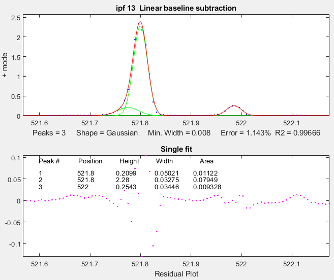
Like iPeak and iSignal, ipf.m starts out by showing the entire signal in the lower panel and the selected region that will be fitted in the upper panel (adjusted by the same cursor controls keys as iPeak and iSignal). After performing a fit (figure on the right), the upper panel shows the data as blue dots, the total model as a red line (ideally overlapping the blue dots), and the model components as green lines. The dotted magenta lines are the first-guess peak positions for the last fit. The lower panel shows the residuals (difference between the data and the model). Important note: Make sure you don't click on the "Show Plot Tools" button in the toolbar above the figure; that will disable normal program functioning. If you do; close the Figure window and start again.

Recent version history. . Version 13.5 adds unconstrained Pearson IV shape (Shift-K); Version 13.3. Added additional baseline correction modes and fixed bug in Voigt shape. Version 13.2: the center of the graph displays "Working..." while the fit is in progress; modified "D" key to save model data to disc as SavedModel.mat. Version 13, November 2017: added new peak shapes, 24 total selectable by single keystroke and 49 total selectable from the "-" menu . Version 12.4: Changed IQR in the bootstrap method to IQR/1.34896, which estimates the RSD without outliers for a normal distribution. Version 11.1 adds  minimum peak width constraint (Shift-W); adds saturation maximum (Shift-M) to ignore points above saturation maximum (useful for fitting flat-top peaks). Version 11 adds polynomial fitting (Shift-o key). Version 10.7 corrects bugs in equal-width Lorentzians (shape 7) and in the bipolar (+ and -) mode. Version 10.5, August 2014 adds Shift-Ctrl-S and Shift-Ctrl-P keys to transfer the current signal to iSignal and iPeak, respectively, if those functions are installed in your Matlab path; Version 10.4, June, 2014. Moves fitting result text to bottom panel of graph. Log mode: (M key) toggles log mode on/off, fits log(model) to log(y). Replaces bifurcated Lorentzian with the Breit-Wigner-Fano resonance peak (Shift-B key); see http://en.wikipedia.org/wiki/Fano_resonance. Ctrl-A selects all; Shift-N negates signal. Version 10 adds multiple-shape models; Version 9.9 adds '+=' key to flip between + (positive peaks only) and bipolar (+/- peaks) modes; Version 9.8 adds Shift-C to specify custom first guess ('start'). Version 9.7 adds Voigt profile shape. Version 9.6 added an additional BaselineMode mode that subtracts a flat baseline without requiring that the signal return to the baseline at both ends of the signal segment. Version 9.5 added exponentially broadened Lorentzian (peak shape 18) and alpha function (peak shape 19);Version 9.4: added bug fix for height of Gaussian/ Lorentzian blend shape; Version 9.3 added Shift-S to save Figure as a png graphic to the current directory. Version 9.2: bug fixes; Version 9.1 added fixed-position Gaussians (shape 16) and fixed-position Lorentzians (shape 17) and a peak shape selection menu ( activated by the '_-' key). 

Demoipf.m is a demonstration script for ipf.m, with a
built-in simulated signal generator. To download these m-files, right-click on these links, select Save Link As..., and click Save. You can also download a ZIP file containing ipf.m, Demoipf.m, and peakfit.m. 

Example 1: Test with pure Gaussian function, default settings of all input arguments..
>> x=[0:.1:10];y=exp(-(x-5).^2);ipf(x,y)
In this example, the fit is essentially perfect, no matter what are the pan and zoom settings or the initial first-guess (start) values. However, the peak area (last fit result reported) includes only the area within the upper window, so it does vary.  (But if there were noise in the data or if the model were imperfect, then all the fit results will depend on the exact the pan and zoom settings).

Example 2: Test with "center" and "window" specified.
>> x=[0:.005:1];y=humps(x).^3;
>> ipf(x,y,0.335,0.39) focuses on first peak
>> ipf(x,y,0.91,0.18) focuses on second peak

Example 3:
>> x=1:.1:1000;y=sin(x).^2;ipf(x,y,843.45,5)
Isolates a  narrow segment toward the end of the signal.

KEYBOARD CONTROLS for Matlab Version 13.5 (Octave version uses different keys for pan and zoom):
 Pan signal left and right...Coarse: < and >
                             Fine: left and right cursor arrow
                             Nudge: [ ]
 Zoom in and out.............Coarse zoom: ?/ and "
                             Fine zoom: up and down
                             arrow keys
 Select entire signal........Crtl-A (Zoom all the way out)
 Resets pan and zoom.........ESC
 Select # of peaks...........Number keys 1-9, or press 0 key to
                             enter number manually
 Select peak shape from menu - (minus or hyphen), then type
                               number or shape vector and Enter
 Select peak shape by key....g
unconstrained Gaussian
                             h equal-width Gaussians
                             Shift-G fixed-width Gaussians
                             Shift-P fixed-position Gaussians
                             Shift-H bifurcated Gaussians
                               
(equal shape, a,z adjust)
                             e Exponential-broadened Gaussian
                              (equal shape, a,z adjust)
                             Shift-R  ExpGaussian (var. tau)
                             j exponential-broadened
                               equal-width Gaussians
                                 (equal shape, a,z adjust)
                             l
unconstrained Lorentzian
                             :; equal-width Lorentzians
                             Shift-[ fixed-position Lorentzians
                             Shift-E Exponential-broadened
                                  Lorentzians
                                 (equal shape, a,z adjust)
                             Shift-L Fixed-width Lorentzians
                               (equal shape, a,z adjust)
                             o LOgistic distribution (Use
                               Sigmoid for logistic function)
                             p Pearson VII (a,z keys adjust shape)
                             Shift-K Pearson IV
, variable asymmetric
                             u exponential pUlse
                               y=exp(-tau1.*x).*(1-exp(-tau2.*x))
                             Shift-U Alpha: y=(x-tau2)./
                                    tau1.*exp(1-(x-tau2)./tau1)
                             s Up Sigmoid (logistic function):
                               y=.5+.5*erf((x-tau1)/sqrt(2*tau2))
                             Shift-D
Down Sigmoid
                              y=.5-.5*erf((x-tau1)/sqrt(2*tau2))
                             ~` Gauss/Lorentz blend (equal shape,
                             Shift-V Voigt profile (a/z adjusts
                                     a,z adjust shape)
                             Shift
-B Breit-Wigner-Fano (equal
                                   
shape a,z adjust)
 Fit.........................f
 Select BaselineMode mode....t  selects none, linear,quadratic,
                               flat or mode(y) baseline mode
 + or +/- peak mode..........+=  Flips between + peaks only and
                                 +/- peak mode
 Invert (negate) signal......Shift-N
 Toggle log y mode OFF/ON....m  Log mode plots and fits
                                log(model) to log(y).
 2-point Baseline............b, then click left and right
                                baseline
 Set manual baseline.........Backspace, then click baseline at
                                        multiple points
 Restore original baseline...|\  to cancel previous background
                                 subtraction
 Cursor start positions......c, then click on each peak
                                position
 Type in start vector........Shift-C Type or Paste start vector
                                     [p1 w1 p2 w2 ...]
 Print current start vector..Shift-Q
 Enter value of 'Extra'......Shift-x, type value (or vector of
                              values in brackets), press Enter.
 Adjust 'Extra' up/down......a,z: 5% change; upper case A,Z:
                                  0.5% change.
 Print parameters & results..q
 Print fit results only......r
 Compute bootstrap stats.....v  Estimates standard deViations
                                of parameters.
 Fit single bootstrap........n  Extracts and Fits siNgle
                                bootstrap sub-sample.
 Plot signal in figure 2.....y
 save model to Disk.......... Save model to disk as
                                SavedModel.mat.                               
  Refine fit.................x Takes best of 10 trial fits
                               (change in line 227 of ipf.m)
 Print peakfit function......w  Print peakfit function with all
                                input arguments
 Save Figure as png file.....Shift-S  Saves as Figure1.png,
                                      Figure2.png, etc.
 Display current settings....Shift-? displays list of current
                                     settings
 Fit polynomial to segment...Shift-o  Asks for polynomial
                                      order 
 Enter minimum width.........Shift-W  Constrains peak widths to
                                      a specified minimum.
 Enter saturation maximum....Shift-M
   Ignores points above a
                                   specified saturation maximum
.
 Switch to iPeak.............Shift-Ctrl-P transfers current
                                          signal to iPeak.m
 Switch to iSignal...........Shift-Ctrl-S transfers current
                                          signal to iSignal.m

(The function ShapeDemo demonstrates the basic peak shapes graphically, showing the variable-shape peaks as multiple lines)

Practical examples with experimental data:

 
1. Fitting weak and noisy peaks. In this example, pan and zoom controls are used to isolate a segment of a chromatogram that contains three very weak peaks near 5.8 minutes The lower plot shows the whole chromatogram and the upper plot shows the segment.  Only the peaks in that segment are subjected to the fit. Pan and zoom are adjusted so that the signal returns to the local baseline at the ends of the segment.


 Pressing T selects BaselineMode mode 1, causing the program to subtract a linear baseline from these data points. Pressing 3, E,
F performs a 3-peak exponentially-broadened Gaussian fit (a common peak shape in chromatography). The A and Z keys are then used to adjust the time constant ("Extra") to obtain the best fit. The residuals (bottom panel) are random and exhibit no obvious structure, indicating that the fit is as good as is possible at this noise level.

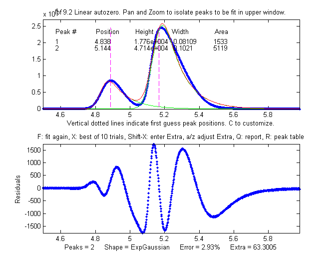
2. Measuring the areas of overlapping peaks. In this example, a sample of room air is analyzed by gas chromatography (data source). The resulting chromatogram (right) shows two slightly overlapping peaks, the first for oxygen and the second for nitrogen. The area under each peak is presumed to be proportional to the gas composition. The perpendicular drop method of measuring the areas gives peak areas in a ratio of 25% and 75%, compared to the actual 21% and 78% composition, which is not very accurate probably because the peaks are visibly asymmetric. But an exponentially-broadened Gaussian (a commonly-encountered peak shape in chromatography) gives a fairly good fit to the data, using ipf.m and adjusting the exponential term with the A and Z keys to get the best fit. The results for a two-peak fit, shown in the ipf.m screen on the right and in the R-key report below, show that the peak areas are in a ratio of 23% and 77%, which is a bit better. With a 3-peak fit, modeling the nitrogen peak as the sum of two closely overlapping peaks whose areas are added together, the curve fit is much better (less than 1% fitting error), and indeed the result in that case is 21.1% and 78.9% - considerably closer the the actual composition.

Percent Fitting Error = 2.9318%  Elapsed time = 11.5251 sec.
 
Peak#  Position   Height    Width     Area
  1     4.8385     17762    0.081094   1533.2
  2     5.1439     47142    0.10205    5119.2

3. The accuracy of peak position measurement can be good even if the fitting error is rather poor. In this example, an experimental high-resolution atomic emission spectrum is examined in the region of the well-known spectral lines of the element sodium. Two lines are found there (figure on the right), and when fit to a unconstrained Lorentzian or Gaussian model, the peak wavelengths are determined to be 588.98 nm and 589.57 nm.
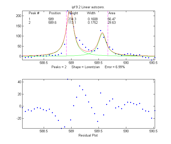
Percent Fitting Error 6.9922%   
Peak#  Position    Height    Width     Area
 
1     588.98     234.34   0.16079    56.473
 
2     589.57     113.18   0.17509    29.63

Compare this to the ASTM recommended wavelengths for this element (588.995 and 589.59 nm) and you can see that the error is no greater than 0.02 nm, which is less than the interval between the data points (0.05 nm). And this is despite the fact that the fit is not particularly good, because the peaks shapes are rather oddly shaped (perhaps by self-absorption, because these particular atomic lines are strongly absorbing as well as strongly emitting). This high degree of absolute accuracy compared to a reliable exterior standard is a testament to the excellent wavelength calibration of the instrument on which these experimental data were obtained, but it also shows that peak position is by far the most precisely measurable parameter in peak fitting, even when the data are noisy and the curve fit is not particularly good. The bootstrap standard deviation estimates calculated by ipf.m for both wavelengths is 0.015 nm (see #17 in the next section), and using the 2 x standard deviation rule-of-thumb would have predicted a probable error within 0.03 nm. (An even lower fitting error can be achieved by fitting to 4 peaks, but the position accuracy of the larger peaks remains virtually unchanged).

4. How many peaks to model? In the second and third examples, the number of peaks in the model was suggested by the data and by the expectations of each of those experiments (two major gasses in air; sodium has a well-known doublet at that wavelength). In the first example, no a priori expectation of number of peaks was available, but the data suggested three obvious peaks, and the residuals were random and unstructured with a 3-peak model, suggesting that no additional models peaks were needed.  In many cases, however, the number of model peaks is not so clearly indicated. For example, in this previously described example, the fitting error keeps getting lower as more peaks are added to the model, yet the residuals remain "wavy" and never become random. Without further knowledge of the experiment, it's impossible to know which are the "real peaks" and what is just "fitting the noise".


Operating instructions for ipf.m (version 13.5). Click here for animated instructions.

  1. At the command line, type ipf(x,y), (x = independent variable, y = dependent variable) or  ipf(datamatrix) where "datamatrix" is a matrix that has x values in row or column 1 and y values in row or column 2. Or if you have only one signal vector y, type ipf(y).  You may optionally add to additional numerical arguments:  ipf(x,y,center,window); where "center" is the desired x-value in the center of the upper window and "window" is the desired  width of that window.

  2. Use the four cursor arrow keys on the keyboard to pan and zoom the signal to isolate the peak or group of peaks that you want to fit in the upper window. (Use the < and > and ? and " keys for coarse pan and zoom and the square bracket keys [ and ] to nudge one point left and right). The curve fitting operation applies only to the segment of the signal shown in the top plot. The bottom plot shows the entire signal. Try not to get any undesired peaks in the upper window or the program may try to fit them. To select the entire signal, press Ctrl-A.

  3. Press the number keys (1 - 9) to choose the number of model peaks, that is, the minimum number of peaks that you think will suffice to fit this segment of the signal. For more than 9 peaks, press 0, type the number, and press Enter.
    |
  4. Select the desired model peak shape. In ipf.m version 13 (November 2017), there are 24 different peaks shapes are available by keystroke, e.g. G=Gaussian, L=Lorentzian, U=exponential pulse, S=sigmoid (logistic function), etc. Press K to see a list of all commands.
      You can also select the shape by number from an even larger menu of 49 shapes by pressing the - (minus) key and selecting the shape by number.  If the peak widths of each group of peaks is expected to be the same or nearly so, select the "equal-width" shapes. If the peak widths or peak positions are known from previous experiments, select the "fixed-width" or "fixed position" shapes. These more constrained fits are faster, easier, and much more stable than regular all-variable fits, especially if the number of model peaks is greater than 3 (because there are fewer variable parameters for the program to adjust - rather than a independent value for each peak). 

  5. A set of vertical dashed lines are shown on the plot, one for each model peak. Try to fine-tune the Pan and Zoom keys so that the signal goes to the baseline at both ends of the upper plot and so that the peaks (or bumps) in the signal roughly line up with the vertical dashed lines, as show in the figures on this Web page. This does not have to be exact.

  6. If you want to allow negative peaks as well as positive peaks, press the + key to flip to the +/- mode (indicated by the +/- sign in the y-axis label of the upper panel. Press it again to return to the + mode (positive peaks only). You can switch between these modes at any time.  To negate the entire signal, press Shift-N.

  7. Press F to initiate the curve-fitting calculation. In version 13.2, the center of the graph displays "Working..." while the fit is in progress. Each time you press F, another fit of the selected model to the data is performed with slightly different starting positions, so that you can judge the stability of the fit with respect to changes in starting first guesses. Keep your eye on the residuals plot and on the "Error %" display. Do this several times, trying for the lowest error and the most unstructured random residuals plot. At any time, you can adjust the signal region to be fit (step 2), the baseline position (step 9 and 10), change the number or peaks (step 3), or peak shape (step 4), then press the F key again to compute another fit. If the fit seems unstable, try pressing the X key a few times (see #13, below).

  8. The model parameters of the last fit are displayed in the upper window. For example, for a 3-peak fit:
    Peak# Position  Height   Width    Area
     1    5.33329   14.8274  0.262253 4.13361
     2    5.80253   26.825   0.326065 9.31117
     3    6.27707   22.1461  0.249248 5.87425
    The column are, left to right: the peak number, peak position, peak height, peak width, and the peak area. (Note: for exponential pulse (U) and sigmoid (S) shapes, Position and Width are replaced by Tau1 and Tau2). Press R to print this table out in the command window. Peaks are numbered from left to right. (The area of each component peak within the upper window is computed using the trapezoidal method and displayed after the width). Pressing Q prints out a report of settings and results in the command window, like so:

    Peak Shape = Gaussian
    Number of peaks = 3
    Fitted range = 5 - 6.64
    Percent Error = 7.4514    Elapsed time = 0.19741 Sec.
    Peak#  Position      Height       Width        Area
    1      5.33329      14.8274     0.262253      4.13361
    2      5.80253       26.825     0.326065      9.31117
    3      6.27707      22.1461     0.249248      5.87425

  9. To select the baseline correction mode, press the T key repeatedly;cycles the baseline correction method to off, linear, quadratic, flat, mode(y), and then back to off. The current method is displayed above the upper panel. When the baseline correction is OFF, peak heights are measured relative to zero. When baseline subtraction is linear, a straight-line baseline connecting the two ends of the signal segment in the upper panel will be automatically subtracted. When baseline subtraction is quadratic, a parabolic baseline connecting the two ends of the signal segment in the upper panel will be automatically subtracted. The mode(y) method subtracts the most common y value (the statistical "mode") from all the points in the selected region. For peak-type signals where the peaks often return to the baseline between peaks, the most common value is usually a good approximation of the baseline even if the signal does not return to the baseline at the ends as required by methods 2 and 3 (graphic example). Use the quadratic baseline correction if the baseline is curved, as in these examples:

    BaselineMode OFF

    Linear BaselineMode

    Quadratic BaselineMode
  10. If you prefer to set the baseline manually, press the B key, then click on the baseline to the LEFT the peak(s), then click on the baseline to the RIGHT the peak(s). The new baseline will be subtracted and the fit re-calculated. (The new baseline remains in effect until you use the pan or zoom controls). Alternatively, you may use the multipoint background correction for the entire signal: press the Backspace key, type in the desired number of background points and press the Enter key, then click on the baseline starting at the left of the lowest x-value and ending to the right of the highest x-value. Press the \ key to restore the previous background to start over.

  11. In some cases it will help to manually specify the first-guess peak positions: press C, then click on your estimates of the peak positions in the upper graph, once for each peak. A fit is automatically performed after the last click. Peaks are numbered in the order clicked. For the most difficult fits, you can type Shift-C and then type in or Paste in the entire start vector, complete with square brackets, e.g. "[pos1 wid1 pos2 wid2 ...]" where "pos1" is the position of peak 1, "wid1" is the width of peak 1, and so on for each peak. The custom start values remain in effect until you change the number of peaks or use the pan or zoom controls. Hint: if you Copy the start vector and keep it in the Paste buffer, you can use the Shift-C key and Paste it back in after changing the pan or zoom controls. Note: It's possible to click beyond the x-axis range, to try to fit a peak whose maximum is outside the x-axis range displayed. This is useful when you want to fit a curved baseline by treating it as an additional peak whose peak position if off-scale (example).

  12. The A and Z keys control the "shape" parameter ('extra') that is used only if you are using the "equal shape" models such as the Voigt profile, Pearson, exponentially-broadened Gaussian (ExpGaussian), exponentially-broadened Lorentzian (ExpLorentzian), bifurcated Gaussian, Breit-Wigner-Fano, or Gaussian/Lorentzian blend. For these models, the shapes are variable with the A and Z keys but are the same for all peaks in the model. For the Voigt profile, the "shape" parameter controls alpha, the ratio of the Lorentzian width to the Doppler width. For the Pearson shape, a value of 1.0 gives a Lorentzian shape, a value of 2.0 gives a shape roughly half-way between a Lorentzian and a Gaussian, and a larger values give a nearly Gaussian shape. For the exponentially broadened Gaussian shapes, the "shape" parameter controls the exponential "time constant" (expressed as the number of points). For the Gaussian/Lorentzian blend and the bifurcated Gaussian shape, the "shape" parameter controls the peak asymmetry (a values of 50 gives a symmetrical peak). For the Breit-Wigner-Fano, it controls the Fano factor. You can enter an initial value of the "shape" parameter by pressing Shift-X , typing in a value, and pressing the Enter key. For multi-shape models, enter a vector of  "extra" values, one for every peak, enclosed in square brackets. For single-shape models, you can adjust this value using the A and Z keys (hold down the Shift key to fine tune). Seek to minimize the Error % or set it to a previously-determined value. Note: if fitting multiple overlapping variable-shape peaks, it's easier to fit a single peak first, to get a rough value for the "shape" parameter parameter, then just fine-tune that parameter for the multipeak fit if necessary.

  13. For situations where the shapes may be different for each peak and you want the computer to determine the best-fit shape for each peak separately, use the shapes with three unconstrained  iterated variables: 30=variable alpha Voigt, 31=variable time constant ExpGaussian (Shift-R), 32=variable shape Pearson, 33=variable percent Gaussian/Lorentzian blend; 49=unconstrained Pearson IV. These models are more time-consuming and difficult, especially for multiple overlapping peaks, especially the Pearson IV, which has 4 iterated variables.

  14. For difficult fits, it may help to press X, which restarts the iterative fit 10 times with slightly different first guesses and takes the one with the lowest fitting error. In version 13.2, the center of the graph displays "Working..." while the fit is in progress. This will take a little longer, obviously. (You can change the number of trials, "NumTrials", in or near line 227 - the default value is 10). The peak positions and widths resulting from this best-of-10 fit then become the starting points for subsequent fits, so the fitting error should gradually get smaller and smaller is you press X again and again, until it settles down to a minimum. If none of the 10 trials gives a lower fitting error than the previous one, nothing is changed. Those starting values remain in effect until you change the number of peaks or use the pan or zoom controls. (Remember: equal-width fits, fixed-width fits, and fixed position shapes are both faster, easier, and much more stable than regular variable fits, so use equal-width fits whenever the peak widths are expected to be equal or nearly so, or fixed-width (or fixed position) fits when the peak widths or positions are known from previous experiments). 
      Here's a simple example where the X key is needed: at the prompt, type ipf(humps). This uses the built-in "humps" function. Try fitting the entire signal with 3 Gaussians (press ctrl-A, 3, G, F). The fit is poor.  Now press X a few times; the fit is much better.

  15. Press Y to display the entire signal full screen without cursors, with the last fit displayed in green. The residual is displayed in red, on the same y-axis scale as the entire signal.

  16. Press M to switch back and forth between log and linear modes. In log mode, the y-axis of the upper plot switches to semilog-y, and log(model) is fit to log(y), which may be useful if the peaks vary greatly in amplitude. 

  17. Press the D key to save the fitting data to disc as SavedModel.mat, containing two matrices: DataSegment (the raw data segment that is fit) and ModelMatrix (a matrix containing each component of the model interpolated to 600 points in that segment).  To place the model data in the workspace, type load SavedModel. To plot DataSegment, type plot(DataSegment(:,1), DataSegment(:,2)). To plot SavedModel, type plot(ModelX,ModelMatrix); each component in the model is plotted in a different color. To plot all of these together, in the format of the upper panel of ipf.m, type plot(DataSegment(:,1), DataSegment(:,2), '.', ModelX, ModelMatrix, ModelX, sum(ModelMatrix')).

  18. Press W to print out the peakfit.m function with all input arguments, including the last best-fit values of the first guess vector. You can copy and paste the peakfit.m function into your own code or into the command window, then replace "datamatrix" with you own x-y matrix variable.

  19. Both ipf.m, and peakfit.m are able to estimate the expected variability of the peak position, height, width, and area from the signal, by using the bootstrap sampling method. This involves extracting 100 bootstrap samples from the signal, fitting each of those samples with the model, then computing the uncertainty of each peak: the standard deviation (RSD) and the relative percent standard deviation (%RSD). Basically this method calculates weighted fits of a single data set, using a different set of different weights for each sample. This process is computationally intensive can take several minutes to complete, especially if the number of peaks in the model and/or the number of points in the signal are high.  

    To activate this process in ipf.m, press the V key. It first asks you to type in the number of "best-of-x" trial fits per bootstrap sample (the default is 1, but you may need higher number here if the fits are occasionally unstable; try 5 or 10 here if the initial results give NaNs or wildly improbable numbers). (To activate this process in peakfit.m, you must use version 3.1 or later and include all six output arguments, e.g. [FitResults, LowestError, residuals, xi, yi, BootstrapErrors]=peakfit...). In version 13.2, the center of the graph displays "Working..." while the fits is in progress. The results are displayed as a table in the command window. For example, here's a three-peak Gaussian fit to some fairly noisy experimental data, followed by a bootstrap statistics calculation:

    Shape= Gaussian   % Fitting Error= 8.1876%   R2= 0.89861
     
    Peak#   Position   Height    Width    Area
        1      573.97     156.96    20.591   3401.6
        2      583.94     146.22    5.3956   839.78
        3      603.94     110.96    16.77    1861.7


    Number of fit trials per bootstrap sample (0 to cancel): 1
    Computing bootstrap sampling statistics....May take several minutes.
     
    Peak #1
    Parameter    Mean      STD    STDIQR    % RSD      % RSDIQR
    ____________  ______  _______  _______ __________ __________
    {'Position'}  573.89  0.33752  0.28748  0.058813    0.050093  
    {'Height'  }  158.53   3.6802   3.0271    2.3215      1.9095  
    {'width'   }  19.038    1.408   1.2717    7.3954      6.6795  
    {'Area'    }  3187.6   194.89   178.79    6.1141      5.6088  
     
    Peak #2
    Parameter    Mean     STD     STDIQR   PercentRSD  % RSDIQR
    ____________  ______  ________  _______  _________  _________
    {'Position'}  583.84  0.098986  0.1007   0.016954    0.017247  
    {'Height'  }  156.03    10.837  11.916    6.9454      7.6372  
    {'width'   }  5.5557   0.26153  0.24418   4.7074      4.3952  
    {'Area'    }  924.28    95.719  76.147    10.356      8.2385  
     
    Peak #3
    Parameter    Mean      STD   STDIQR  PercentRSD   % RSDIQR
    ____________  ______  _______ _______ __________ ___________
    {'Position'}   603.4  0.36056 0.33927  0.059754     0.056227  
    {'Height'  }  113.24   3.9028  4.3535    3.4465      3.8445  
    {'width'   }  16.128   1.2027  1.2781     7.457      7.9247  
    {'Area'    }  1843.3   79.733  87.735    4.3256      4.7598  
    Elapsed time is 10.65 seconds.

Note that, despite the noise in the data and the 8% fitting error, the bootstrap relative standard deviations are not so bad, especially for peak positions and heights. Notice that the RSD of the peak position is best (lowest), followed by height and width and area. This is a typical pattern, seen before. Also, be aware that the reliability of the computed variability depends on the assumption that the noise in the signal is representative of the average noise in repeated measurements. If the number of data points in the signal is small, these estimates can be very approximate.

If the RSD and the RSDIQR are roughly the same (as in the example above), then the distribution of bootstrap fitting results is close to normal and the fit is stable. If the RSD is substantially greater than RSD IQR, then the RSD is biased high by "outliers" (obliviously erroneous fits that fall far from the norm), and in that case you should use the RSD IQR rather than the RSD, because the IQR is much less influenced by outliers. (Alternatively, you could use another model or a different data set to see if that gives more stable fits).

A likely pitfall with the bootstrap method when applied to iterative fits is the possibility that one (or more) of the bootstrap fits will go astray, that is, will result in peak parameters that are wildly different from the norm, causing the estimated variability of the parameters to be too high. For that reason, in ipf 12.3 and later, two measures of uncertainty are calculated: (a) the regular standard deviation (STD) and (b) the standard deviation estimated by dividing the interquartile range (IQR) by 1.34896, which is labeled RSD (IQR). The IQR is more robust to outliers that STD. For a normal distribution, the interquartile range is on average equal to 1.34896 times the standard deviation. If one or more of the bootstrap sample fits fails, resulting in a distribution of peak parameters with large outliers, the regular STD will be much greater that the IQR. In that case, a more realistic estimate of variability is IRQ/1.34896. It's best to try to increase the fit stability by choosing a better model (e.g. using an equal-width or fixed-width model, or a fixed-position shape, if appropriate), adjusting the fitted range (pan and zoom keys), the background subtraction (T or B keys), or the start positions (C key), and/or selecting a higher number of fit trials per bootstrap (which will increase the computation time). As a quick preliminary test of bootstrap fit stability, pressing the N key will perform a single iterative fit to a random bootstrap sub-sample and plot the result; do that several times to see whether the bootstrap fits are stable enough to be worth computing a 100-sample bootstrap. Note: it's normal for the stability of the bootstrap sample fits (N key: click here for animation) to be poorer than the full-sample fits (F key; click here for animation), because the latter includes only the variability caused by changing the starting positions for one set of data and noise, whereas the N and V keys aim to include the variability caused by the random noise in the sample by fitting bootstrap sub-samples. Moreover, the best estimates of the measured peak parameters are those obtained by the normal fits of the full signal (F and X keys), not the means reported for the bootstrap samples (V and N keys), because there are more independent data points in the full fits and because the bootstrap means are influenced by the outliers that occur more commonly in the bootstrap fits. The bootstrap results are useful only for estimating the variability of the peak parameters, not for estimating their mean values. The N and V keys are also very useful way to determine if you are using too many peaks in your model; superfluous peaks will be very unstable when N is press repeatedly and will have much higher standard deviation of its peak height when the V key is used.
19. Shift-o fits a simple polynomial (linear, quadratic, cubic, etc) to the segment of the signal displayed in the upper panel and displays the polynomial coefficients (in descending powers) and the R2.

20.
If some peaks are saturated and have a flat top (clipped at a maximum height), you can make the program ignore the saturated points by pressing Shift-M and entering the maximum Y values to keep. Y values above this limit will simply be ignored; peaks below this limit will be fit as usual.

21. To constrain the model to peaks above a certain width, press Shift-W and enter the minimum peak with allowed.
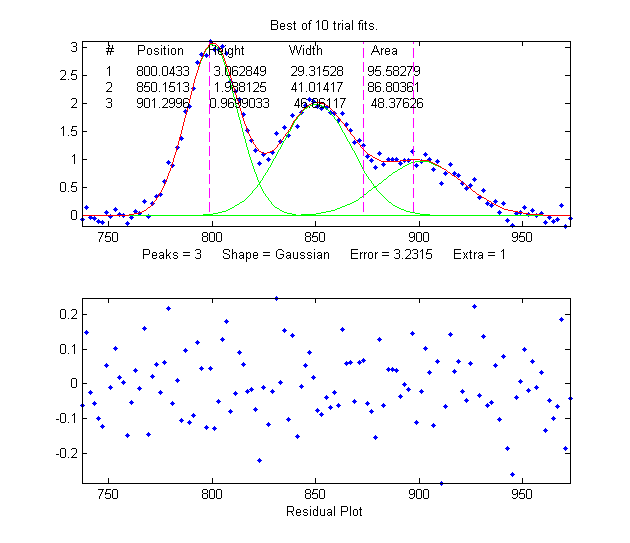
Demoipf.m

Demoipf.m is a demonstration script for ipf.m, with a built-in simulated signal generator. The true values of the simulated peak positions, heights, and widths are displayed in the Matlab command window, for comparison to the FitResults obtained by peak fitting. The default simulated signal contains six independent groups of peaks that you can use for practice: a triplet near x = 150, a singlet at 400, a doublet near 600, a triplet near 850, and two broad single peaks at 1200 and 1700. Run this demo and see how close to the actual true peak parameters you can get. The useful thing about a simulation like this is that you can get a feel for the accuracy of peak parameter measurements, that is, the difference between the true and measured values of peak parameters. To download this m-file, right-click on the links, select Save Link As..., and click Save. To run it it, place both ipf.m and Demoipf in the Matlab path, then type Demoipf at the Matlab command prompt.

An example of the use of this script is shown on the right.  Here we focus in on the 3 fused peaks located near x=850.  The true peak parameters (before the addition of the random noise) are:

Position     Height        Width     Area
800            3           30       95.808
850            2           40       85.163
900            1           50       53.227

When these peaks are isolated in the upper window and fit with three Gaussians, the results are

Position     Height       Width       Area 
800.04       3.0628       29.315     95.583
850.15       1.9881       41.014     86.804
901.3        0.9699       46.861     48.376

So you can see that the accuracy of the measurements are excellent for peak position, good for peak height, and least good for peak width and area.  It's no surprise that the least accurate measurements are for the smallest peak with the poorest signal-to-noise ratio. Note: the predicted standard deviation of these peak parameters can be determined by the bootstrap sampling method, as described in the previous section. We would expect that the measured values of the peak parameters (comparing the true to the measured values) would be within about 2 standard deviations of the true values listed above).

Demoipf2.m is identical, except that the peaks are superimposed on a strong curved baseline, so you can test the accuracy of the baseline correction methods (# 9 and 10, above).

Execution time

By execution time I mean the time it takes for one fit to be performed, exclusive of plotting or printing the results. The biggest factors that determine the execution time are (a) the speed of the computer, (b) the number of peaks, and (c) the peak shape:
a) The execution time can vary over a factor of 4 or 5 or more between different computers, (e.g. a small laptop with 1.6 GHz, dual core Athlon CPU with 4 Gbytes RAM, vs a desktop with a 3.4 GHz i7 CPU with 16 Gbytes RAM).  Run the Matlab "bench.m" benchmark test to see how your computer stacks up.

b) The execution time increases with the product of the number of peaks in the model times the number of iterated variables per peak. (See PeakfitTimeTest.m).

c) The execution time varies greatly (sometimes by a factor of 100 or more) with the peak shape, with the exponentially-broadened shapes being the slowest and the fixed-width shapes being the fastest.  See PeakfitTimeTest2.m and PeakfitTimeTest2a.m  The equal-width and fixed-width shape variations are always faster.  

d) The execution time increases directly with NumTrials in peakfit.m. The "Best of 10 trials" function (X key in ipf.m) takes about 10 times longer than a single fit.  
Other factors that are less important are the number of data points in the fitted region (but only if the number of data points is very large; for example see PeakfitTimeTest3.m) and the starting values (good starting values can reduce execution time slightly; PeakfitTimeTest2.m and PeakfitTimeTest2a.m have examples of that). Note: some of these scripts need DataMatrix2 and  DataMatrix3, which you can download from http://tinyurl.com/cey8rwh.

TimeTrial.txt is a text file comparing the speed of 18 different signal processing tasks running on several different hardware configurations: Windows 10, 64 bit, 3 GHz core i5, with 12 GBytes RAM computer, using Matlab 7.8 R2009a, Matlab 2017b Home, Matlab 2020b, Matlab Online R2018b in Chrome, Matlab Mobile on an iPad), and on Octave 3.6.4. The Matlab/Octave code that generated this is TimeTrial.m, which runs all of the tasks one after the other and prints out the elapsed times for your machine plus the times previously recorded for each tasks on each of the five software systems. The main conclusions that can be drawn from all these results are: (1) All the versions of Matlab, including the online and iPad ones, provide computational speeds that are mostly with a factor of two of each other, and (2) Octave is somewhat slower than any Matlab version.


Hints and Tips

  1. If the fit fails completely, returning all zeros, the data may be formatted incorrectly. The independent variable ("x") and the dependent variable ("y") must be separate vectors or columns of a 2 x n matrix, with x in the first row or column. Or it may be that first guesses ("start") need to be provided for that particular fit.
  2. It's best not to smooth your data prior to curve fitting. Smoothing can distort the signal shape and the noise distribution, making it harder to evaluate the fit by visual inspection of the residuals plot.  Smoothing your data beforehand makes it impossible to achieve the goal of obtaining a random unstructured residuals plot and it increases the chance that you will "fit the noise" rather that the actual signal. The bootstrap error estimates are invalid if the data are smoothed.
  3. The most important factor in non-linear iterative curve fitting is selecting the underlying model peak function, for example, Gaussian, Equal-width Guardians, Lorentzian, etc. (Some examples of this). It's worth spending some time finding and verifying a suitable function for your data. In particular, if the peak widths of each group of peaks is expected to be the same or nearly so, select the "equal-width" shapes; equal-width fits (available for the Gaussian and Lorentzian shapes) are faster, easier, and much more stable than regular variable-width fits.  But it's important to understand that a good fit is not by itself proof that the shape function you have chose it the correct one; in come cases the wrong function can give a fit that looks perfect. For example, this fit of a real data set to a 5-peak Gaussian model has a low percent fitting error and the residuals look random - usually an indicator of a good fit.  But in fact in this case the model is wrong; that data came from an experimental domain where the underlying shape is fundamentally non-Gaussian but in some cases can look very like a Gaussian. It's important to get the model right for the data and not depend solely on the goodness of fit.
  4. You should always use the minimum number of peaks that adequately fits your data. (Some examples of this). Using too many peaks will result in an unstable fit - the green lines in the upper plot, representing the individual component peaks, will bounce around wildly for each repeated fit, without significantly reducing the Error. A very useful way to determine if you are using too many peaks in your model is to use the N key (see #10, below) to perform a single fit to a bootstrap sub-sample of points; superfluous peaks will be very unstable when N is press repeatedly. (You can get better statistics for this test, at the expense of time, by using the V key to compute the standard deviation of 100 bootstrap sub-samples).
  5. If the peaks are superimposed on a background or baseline, that has to be accounted for before fitting, otherwise the peak parameters (especially height, width and area) will be inaccurate. Either subtract the baseline from the entire signal using the Backspace key (# 10 in Operating Instructions, above) or use the T key to select one of the 5 automatic baseline correction modes (# 9 in Operating Instructions, above).
  6. This program uses an iterative non-linear search function ("modified Simplex") to determine the peak positions and widths that best match the data. This requires first guesses for the peak positions and widths. (The peak heights don't require first guesses, because they are linear parameters; the program determines them by linear regression). The default first guesses for the peak positions are made by the computer on the basis of the pan and zoom settings and are indicated by the magenta vertical dashed lines. The first guesses for the peak widths are computed from the Zoom setting, so the best results will be obtained if you zoom in so that the particular group of peaks is isolated and spread out as suggested by the peak position markers (vertical dashed lines).
  7. If the peak components are very unevenly spaced, you might be better off entering the first-guess peak positions yourself by pressing the C key and then clicking on the top graph where you think the peaks might be. None of this has to be exact - they're just first guesses, but if they are too far off it can throw the search algorithm off. You can also type in the first guesses for position and width manually by pressing Shift-C).
  8. Each time you perform another iterative fit (e.g. pressing the F key), the program adds small random deviations to the first guesses, in order to determine whether an improved fit might be obtained with slightly different first guesses. This is useful for determining the robustness or stability of the fit with respect to starting values. If the error and the values of the peak parameters vary slightly in a tight region, this means that you have a robust fit (for that number of peaks). If the error and the values of the peak parameters bounces around wildly, it means the fit is not robust (try changing the number of peaks, peak shape, and the pan and zoom settings), or it may simply be that the data are not good enough to be fit with that model. Try pressing the X key, which takes the best of 10 iterative fits and also uses those best-fit values as the starting first guesses for subsequent fits. So each time you press X, if any of those fits yield a fitting error less that the previous best, that one is taken as the start for the next fit.  As a result, the fits tend to get better and better gradually as the X key is pressed repeatedly. Often, even if the first fit is terrible, subsequent X-key fits will improve considerably.
  9. The variability in the peak parameters from fit to fit using the X or F keys is only an estimate of the uncertainty caused by the curve fitting procedure (but not of the uncertainty caused by the noise in the data, because this is only for one sample of the data and noise; for that you need the N key fits).
  10. To examine the robustness or stability of the fit with respect to random noise in the data, press the N key. Each time you press N, it will perform an iterative fit on a different subset of data points in the selected region (called a "bootstrap sample"). If that gives reasonable-looking fits, then you can go on to compute the peak error statistics by pressing the V key.  If on the other hand the N key gives wildly different fits, with highly variable fitting errors and peak parameters, then the fit is not stable, and you might try the X key to take the best of 10 fits and reset the starting guesses, then press N again. In difficult cases, it may be necessary to increase the number of trials when asked (but that will increase the time it takes to complete), or if that does not help, use another model or a better data set. (The N and V keys are a good way to evaluate a multi-peak model for the possibility of superfluous peaks, see # 4 above).
  11. If you don't find the peak shape you need in this program, look at the next section , or write me and I'll see what I can do.
  12. If you try to fit a very small independent variable (x-axis) segment of a very large signal, say, a region that that is only 1000th or less of the entire x-axis range, you might encounter a problem with unstable fits. If that happens, try subtracting a constant from x, then perform the fit, then add in the subtracted amount to the measured x positions.
  13. If there are very few data points on the peak, it might be necessary to reduce the minimum width (set by minwidth in peakfit.m or Shift-W in ipf.m) to zero or to something smaller than the default minimum (which defaults to the x-axis spacing between adjacent points).
  14. Difference between in the F, X, N, and V keys:

Live script Peak Fitting Tool

Like the other Live Scripts described above, PeakFittingTool.mlx has a file browser button in line 1 and a pair of sliders in lines 4 and 5 for setting the desired segment to work on. But before opening a file, it's a good idea to temporarily de-select the "FitPeaks" check-box in line 14, then when you have set all the other controls, click it back on. That way you will avoid waiting for unnecessary curve fit operations until the appropriate settings are complete. (In challenging cases, curve fitting operations can be slow and can take several seconds in difficult cases).


Adjust the startpc and endpc sliders in lines 4 and 5 to isolate groups of closely-spaced peaks that can be fit together. Try to spread them out as evenly as possible, as shown in the figure above. (If all the peaks are well separated and do not overlap, you may be between off using the Peak Detector Tool (Peakdetector.mlx), which also has a peak fitting function).

The "PreProcess" check box (line 7) allows for some optional preliminary pre-processing.

The SymmetrizeFactor slider in line 8 preforms "symmetrization" or "de-tailing" for peaks that are skewed by exponential broadening, by means of the first-derivative addition. Increase the value of SymmetrizeFactor until the peak is as narrow as possible without the trailing edge falling below the baseline.

The SmoothWidth and NumPasses sliders (lines 9 and 10) permit sliding average smoothing on the signal, which is useful for cases where high-frequency noise obscures the peaks.

The VerticalShift slider (line 11) allows for positive and negative shift in the baseline position, to compensate for baseline offset.

The PeakShape drop-down menu allows you to select the peak shape of the fitting model.
NumPeaks
sets the number of peaks in the model. NumTrials, restarts the fitting process "NumTrials" times with slightly different start values and selects the best one (with lowest fitting error).
NumTrials
can be any positive integer. In many cases, NumTrials=1 will be sufficient, but if that does not give consistent results, increase it until the result are stable.
The extra slider is used to fine-tune the certain peak shapes, e.g., the Pearson, exponentially-broadened Gaussian, and Gaussian/Lorentzian blend. Adjust this to minimize the fitting error.

After all of these settings have been made, then you can activate the FitPeaks check-box, a fit will be performed, and the resulting peak table displayed in the right-hand panel, as in the graphic above. Thereafter, any changes in the setting will cause an immediate recalculation of the curve fit.

In difficult cases, better results can be obtained if you specify the estimated positions of the peaks, especially if the peaks are very irregularly spaced or if some peaks appear only as shoulders or bulges rather than as distinct peaks. Select the SetStart check box and adjust the sliders to the predicted relative peak positions, for each peak in the model in lines 19 to 26.
The length of these sliders represents the x-axis range displayed in the figure.

If the baseline for the group of peaks is offset from zero, you can correct that by using the BaselineShift slider in line 28. If the baseline for the group of peaks is tilted or curved, you can use the BaselineSelection menu in line 27 to choose a baseline correction that attempts to estimate the baseline from the edges of the signal range.

The Bipolar check box (line 29) controls whether to display both positive and negative signal values in the graphic or only positive values.
 
Additional model peak shapes may easily be added to the PeakShape menu by selecting other shapes form the list of predefined shapes and their corresponding number in the list at the top of this page, adding that name and number to the others in the switch/case statement in lines 52-73, then adding that new shape to the drop-down menu on line 15.
Just follow that pattern of the shapes already there.

Another example of Peak Fitting Tool shows it fitting a group of weak peaks in the middle of a much larger signal (chrom.csv), in this case using the exponentially broadened Gaussian shape and the "Tilted mode" baseline correction (line 27). 

In fitting asymmetrical peaks what have an exponential skew, you can either try to remove the asymmetry by using the
SymmetrizeFactor slider (example) followed by fitting a symmetrical peak shape or by selecting an exponentially broadened peak shape (example); both approaches can yield similar results as in these examples, but the former method is often faster.

Note: you can double-click sliders to change their ranges if the initial range is insufficient.


Extracting the equations for the best-fit models

The equations for the peak shapes are in the peak shape menu in ipf.m, isignal.m, and ipeak.m. Here are the expressions for the shapes that are expressed mathematically rather than algorithmically:

Gaussian:          y =exp(-((x-pos)/(0.60056120439323*width)) ^2)
Lorentzian:        y =1/(1+((x-pos)/(0.5*width))^2)
Logistic:          y =exp(-((x-pos)/(.477*wid))^2); y=(2*n)/(1+n)
Lognormal:         y = exp(-(log(x/pos)/(0.01*wid)) ^2)
Pearson:           y =1/(1+((x-pos)/((0.5^(2/m))*wid))^2)^m
Breit-Wigner-Fano: y =((m*wid/2+x-pos)^2)/(((wid/2)^2)+(x-pos)^2)
Alpha function:    y =(x-spoint)/pos*exp(1-(x-spoint)/pos)
Up Sigmoid:        y =.5+.5*erf((x-tau1)/sqrt(2*tau2))
Down Sigmoid       y =.5-.5*erf((x-tau1)/sqrt(2*tau2))
Gompertz:          y =Bo*exp(-exp((Kh*exp(1)/Bo)*(L-t) +1))
FourPL:            y = 1+(miny-1)/(1+(x/ip)^slope)
OneMinusExp:       y = 1-exp(-wid*(x-pos))
EMG (shape 39)     y = s*lambda*sqrt(pi/2)*exp(0.5*(s*lambda)^2-lambda*(t-mu))*erfc((1/sqrt(2))*(s*lambda-((t-mu)/s)))

The peak parameters (height, position, width, etc) that are returned by the FitResults displayed on the graph and in the command window. For example, if you fit a set of data to a single Gaussian and get

    Peak#   Position    Height   Width      Area
     1      0.30284     87.67   0.23732    22.035

then the equation would be

y = 87.67*exp(-((x-0.30284)/(0.60056120439323*0.23732))^2)

If you specify a model of more then one peak, then the equation is the sum of each peak in the model. For example, fitting the built-in Matlab "humps" function using a model of 2 Lorentzians

>> x=[0:.005:2];y=humps(x);[FitResults,GOF]=peakfit([x' y'],0,0,2,2)

    Peak#    Position   Height    Width     Area 
      1      0.3012   96.9405    0.1843   24.9270
      2      0.8931   21.1237    0.2488    7.5968

The equation would be

y = 96.9405*(1/(1+((x-0.3012)/(0.5*0.1843))^2)) + 21.1237*(1//(1+((x-0.8931)/(0.5*0.2488))^2))


It's also possible to use multiple shapes in one fit, by specifying the peak shape parameter as a vector. For example, you could fit the first peak of the "humps" function with a Lorentzian and the second peak with a Gaussian by using [2 1] as the shape argument.

>> x=[0:.005:2];y=humps(x);peakfit([x' y'],0,0,2,[2 1])

    Peak#    Position   Height    Width      Area 
      1      0.3018   97.5771    0.1876   25.4902
      2      0.8953   18.8877    0.3341    6.7180

In that case the expression would be y = Lorentzian  + Gaussian:

y = 97.5771*(1/(1+((x-0.3018)/(0.5*0.1876))^2)) + 18.8877*exp(-((x-0.8953)/(0.60056120439323*0.3341))^2)

Note: to obtain the a digitally sampled model, use peakfit's 6th and 7th output parameters, xi and yi, which return a 600-point interpolated model. Type plot(xi,yi) to plot each model peak separately or plot(xi,yi(1,:)) to plot peak 1.


How to add a new peak shape to peakfit.m, ipf.m, iPeak, or iSignal

  It's easier than you think to add your own custom peak shape to peakfit.m (or to those interactive functions that use peakfit.m, such as ipf.m, iSignal, or iPeak), assuming that you have a mathematical expression for your shape. The easiest way is to modify an existing peak shape that you do not plan to use, replacing it with your new function. Pick a shape to sacrifice that has the same number of variables and constraints are your new shape. For example, if your shape has two iterated parameters (e.g., variable position and width), you could modify the Gaussian, Lorentzian, or triangular shape (number 1, 2 or 21, respectively). If your shape has three iterated variables, use shapes like 31 (Shift-R), 32, 33, or 34. If your shape has four iterated variables, use shape 49 ("Pearson IV", Shift-K). If your shape has an 'extra' parameter, like the equal-shape Voigt, Pearson, BWF, or blended Gaussian/ Lorentzian, use one of those. If you need an exponentially modified shape, use the exponentially modified Gaussian (5 or 31) or Lorentzian (18). If you need equal widths or fixed widths, etc., use one of those shapes. This is important; you must have the same number of variables and constraints, because the structure of the code is different for each class of shapes.

There are just two required steps to the process:

1. Let's say that your shape has two iterated parameters and you are going to sacrifice the triangular shape, number 21. Open peakfit.m or ipf.m in the Matlab editor and re-write the old shape function ("triangular", located near line 3672 in ipf.m - there is one of those functions for each shape - by changing name of the function and the mathematics of the assignment statement (e.g. g = 1-(1./wid).*abs(x-pos);). You can use the same variables ('x' for the independent variable, 'pos' for peak position, 'wid' for peak width, etc.) Scale your function to have a peak height of 1.0 (e.g. after computing y as a function of x, divide by max(y)).

2. Use the search function in Matlab to find all instances of the name of the old function and replace it with the new name, checking "Wrap around" but leaving "Match case" and "Whole word" unchecked in the Search box. If you do it right, for example, all instances of "triangular" and all instances of "fittriangular' will be modified with your new name replacing "triangular". Save the result (or Save as... with a modified file name).

That's it! Your new shape will now be shape 21 (or whatever was the shape number of the old shape you sacrificed). In ipf.m, it will be activated by the same keystroke used by the old shape (e.g. Shift-T for the triangular, key number 84), and in iSignal and in iPeak, the menu of peak shapes will have been modified by the search and replace in step 2.

If you wish, you can change the keystroke assignment in ipf.m; first, find a key or Shift-Key that is not yet assigned (and which gives an "UnassignedKey" error statement when you press it with ipf.m running). Then change the old key number 84 to that unassigned one in the big "switch double(key)," case statement near the beginning of the code. But it's simpler just to use the old key. 

Perhaps you need something more complex, like a combination model with some parameters fixed, some equal to others, some with upper and lower bounds, and some unconstrained - the possibilities are nearly limitless. But by studying the differences between the the various models that my programs already contains, you may be able to figure out how to construct a code that works.  If you do come up with something that works, and you think it would be useful to other people, let me know and I''ll add it, with attribution to you, of course.

indexprevious next
Tom O'Haver
Professor Emeritus
Department of Chemistry and Biochemistry
The University of Maryland at College Park
toh@umd.edu
http://www.wam.umd.edu/~toh

This page is part of "A Pragmatic Introduction to Signal Processing", created and maintained by Prof. Tom O'Haver , Department of Chemistry and Biochemistry, The University of Maryland at College Park. Comments, suggestions and questions should be directed to Prof. O'Haver at toh@umd.edu.

Last update, June, 2023 Number of unique visits since May 17, 2008:

counter create hit