Resource selection functions
Elie Gurarie and Eric Palm
1 Objectives
In this lesson we will analyze caribou resource selection with respect to elevation, time since fire and distance to roads. We’ll start with a simple point-based resource selection function (RSF), and then move to a path-based step selection function (SSF). The basic idea is to figure out what habitat covariates caribou are selecting (or avoiding). Assuming that some resources are actively selected over other resources, the RSF attempts to quantify that selection for (or avoidance of) each. The strategy is simple: - Collect data on used locations - Define and collect data on available (but not necessarily used) locations - Perform a logistic regression.
1.1 Packages and functions
We will use the following packages:
adehabitatHR- for calculating home rangesamt- brand new package for step-selection functionssjPlot- for simple plotting of model coefficientssp- for spatial points
pcks <- list("sp", "sf", "raster", "rgdal", "rgeos", "ggmap", "adehabitatHR", "sjPlot")
sapply(pcks, require, char = TRUE)
## [1] TRUE TRUE TRUE TRUE TRUE TRUE TRUE TRUE2 Resource selection function
The strategy for perfroming an RSF is as follows:
- Find used locations
- Define availabily and sample available locations
- Extract environmental covariates for both
- Perform logistic regression on the Used vs. Available designation with the covariates as explanatory factors.
In math, the RSF is: \[w(X) = \exp(\beta_1 x_1 + \beta_2 x_2 + \beta_3 x_3 + ...)\] - Positive \(\beta\)’s = preference - Negative \(\beta\)’s = avoidance
Where (it turns out) the logistic regression coefficients estimate those \(\beta\)’s.
Let’s start by loading and plotting our habitat data:
load("./_data/fmch.habitat.rda")
plot(fmch.habitat)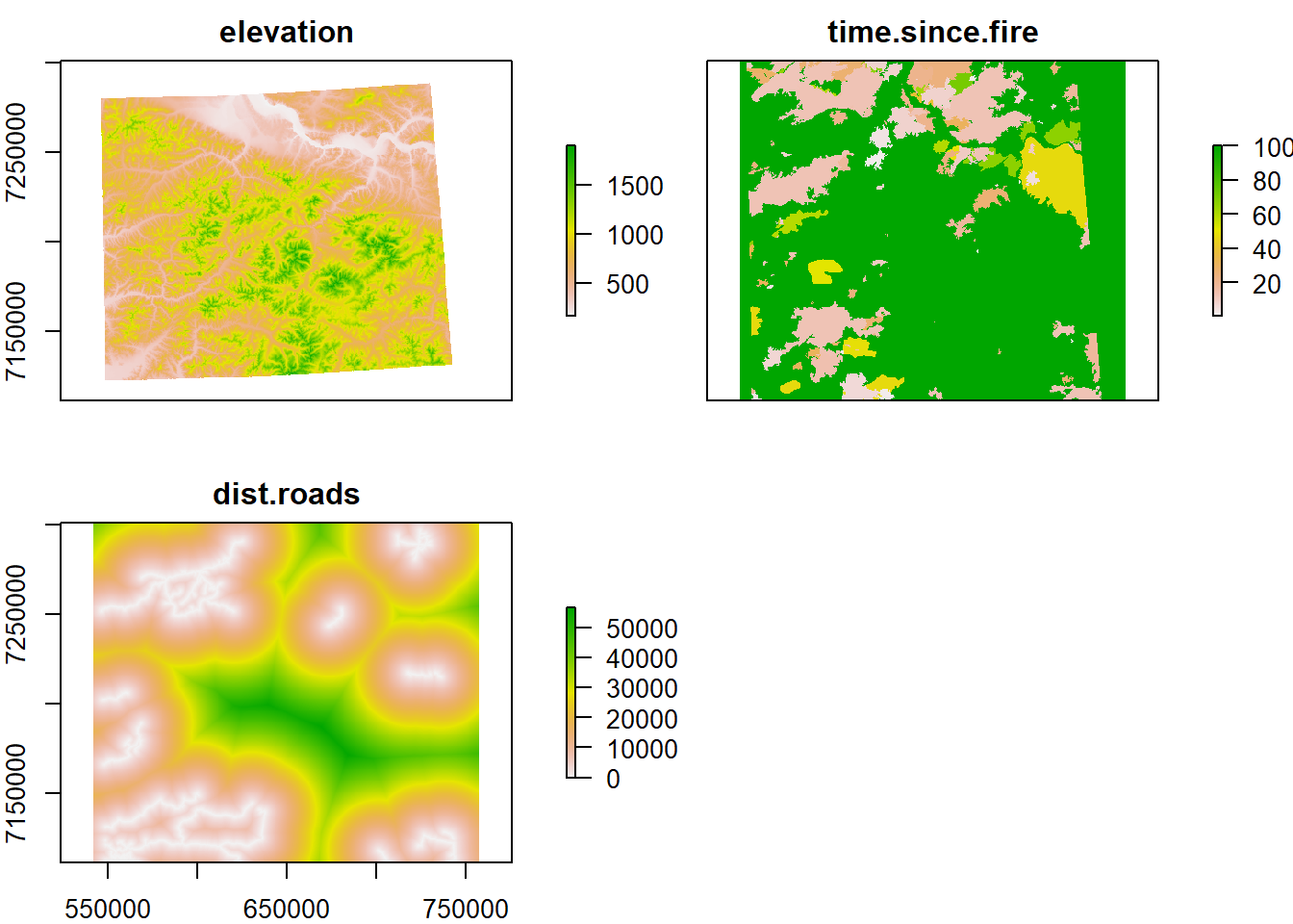
2.1 Defining availability
There are many ways to define availability. We could calculate a minimum convex polygon (MCP), a kernel density estimate home range (KDE), a brownian bridge movement model (BBMM), a Kriged ocurrence distribution, and more. Although our caribou data is not appropriate for an MCP or any type of “home range” because they are displaying no spatial central tendency during our sampling period, we’re going to do it anyway, because it is the simplest way to define availability and may be appropriate for some of your data.
This chunk of code loads the caribou data frame, converts it to a SpatialPointsDataFrame, and plots the caribou object over elevation, constructs an MCP that encompasses 100% of the used points, and plots the MCP:
require(adehabitatHR)
load("./_data/caribou.df.rda")
caribou.sp <- SpatialPoints(caribou.df[, c("x", "y")], proj4string = CRS("+proj=utm +zone=6 +ellps=WGS84 +datum=WGS84 +units=m +no_defs"))

plot(fmch.habitat[[1]])
points(caribou.sp, pch = 19, cex = 0.5, col = rgb(0, 0, 0, 0.2))

# compute mcp
caribou.mcp <- mcp(caribou.sp, 100)
lines(caribou.mcp, col = "red", lwd = 2)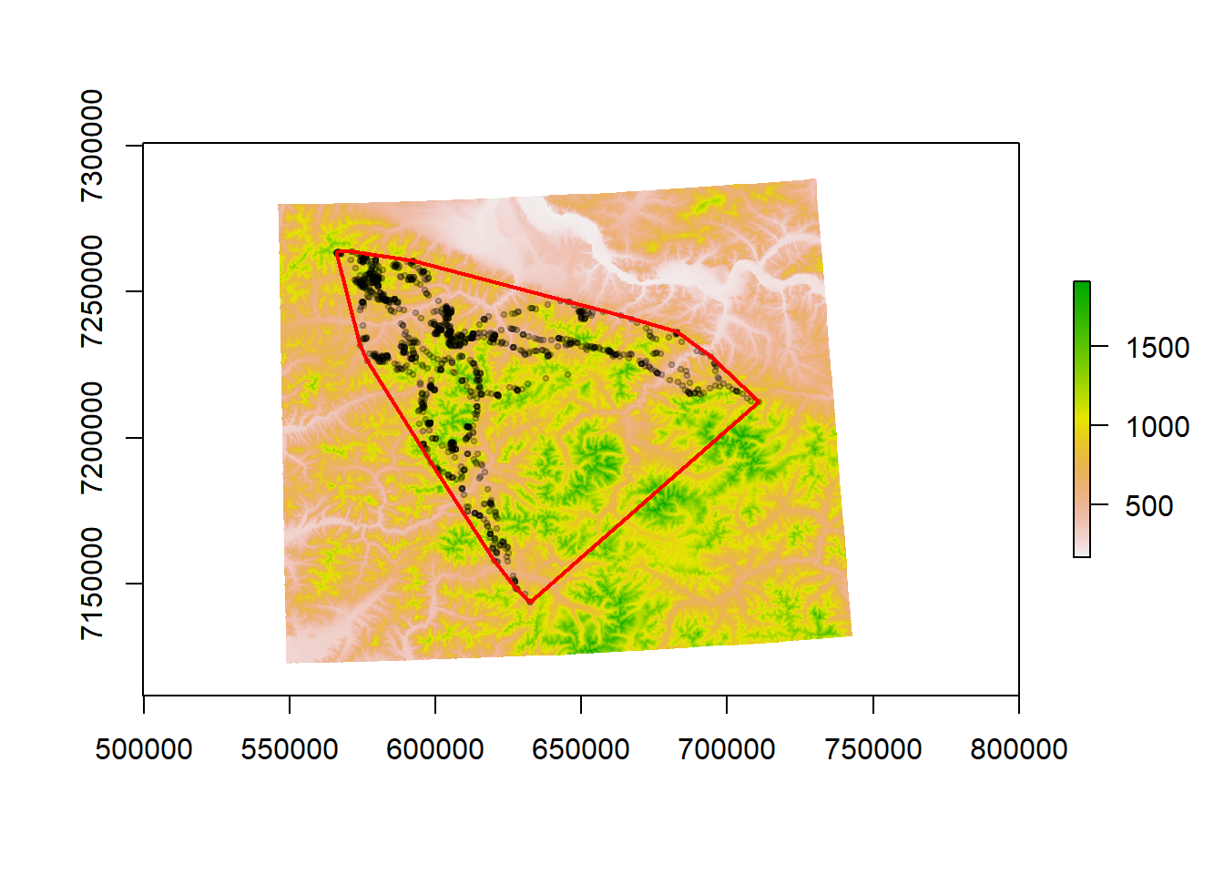
Now obtain some random points from within the MCP. The key function here is spsample. You should get a number comparable to the number of observations (often larger). ** Note - we also subsample the total movement data set - in an ad hoc battle against autocorrelations. This is some major under-the-rug-sweeping**:
xy.obs <- caribou.df[sample(1:nrow(caribou.df), 200), c("x", "y")]
xy.random <- spsample(caribou.mcp, 1000, "random")@coords
plot(xy.random, asp = 1, col = "darkblue", pch = 19, cex = 0.5)
points(xy.obs, pch = 19, col = "orange", cex = 0.5)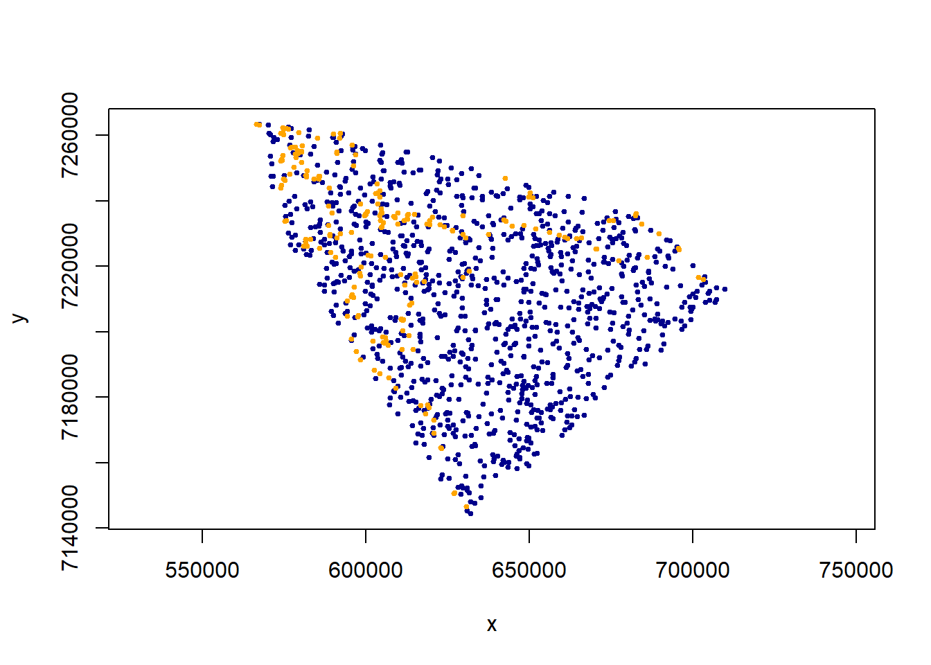
We stack the used and available points, and label them and Used: TRUE/FALSE:
Data.rsf <- data.frame(X = c(xy.obs[, 1], xy.random[, 1]),
                                             Y = c(xy.obs[, 2], xy.random[, 2]),
                                             Used = c(rep(TRUE, nrow(xy.obs)), rep(FALSE, nrow(xy.random))))
Now, we extract the two variables we have for the used and available points:
Data.rsf$elevation <- raster::extract(fmch.habitat[[1]], Data.rsf[, 1:2])
Data.rsf$time.since.fire <- raster::extract(fmch.habitat[[2]], Data.rsf[, 1:2])
Data.rsf$dist.roads <- raster::extract(fmch.habitat[[3]], Data.rsf[, 1:2])
head(Data.rsf)
## X Y Used elevation time.since.fire dist.roads
## 1 682404.0 7235426 TRUE 840.6854 100 11588.356
## 2 579000.9 7255520 TRUE 1088.5463 100 3420.526
## 3 580933.4 7226184 TRUE 887.9063 100 24492.040
## 4 600647.5 7223435 TRUE 1160.4224 100 27294.322
## 5 580365.6 7255142 TRUE 1007.6059 100 2302.173
## 6 660838.3 7228935 TRUE 762.7285 100 19525.6242.2 Visually compare used and available points
boxplot(elevation ~ Used, data = Data.rsf, main = "elevation")
boxplot(time.since.fire ~ Used, data = Data.rsf, main = "time since fire")
boxplot(dist.roads ~ Used, data = Data.rsf, "distance to roads")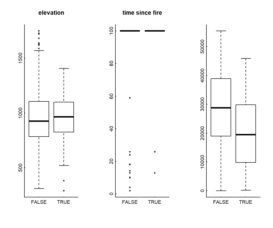
You can see that nearly all used and available points are located in “unburned” areas with a value of 100 years (which we assigned earlier).
3 Fitting an RSF
To estimate the RSF, we simply use a logistic regression. simple glm with a “binomial” link, because our used variable is “TRUE” or “FALSE”
RSF.fit <- glm(Used ~ scale(elevation) + scale(time.since.fire) + scale(dist.roads), data = Data.rsf, family = "binomial")Here are the coefficients of the model:
summary(RSF.fit)$coef## Estimate Std. Error z value Pr(>|z|)
## (Intercept) -1.7904921 0.08938674 -20.030846 2.965760e-89
## scale(elevation) 0.2849544 0.09194635 3.099138 1.940847e-03
## scale(time.since.fire) 0.1898490 0.09535025 1.991069 4.647327e-02
## scale(dist.roads) -0.7959402 0.09131543 -8.716382 2.872326e-18Plotting the coefficients is easy with the sjPlot package (which, however, can by fussy to install!):
require(sjPlot)
plot_model(RSF.fit)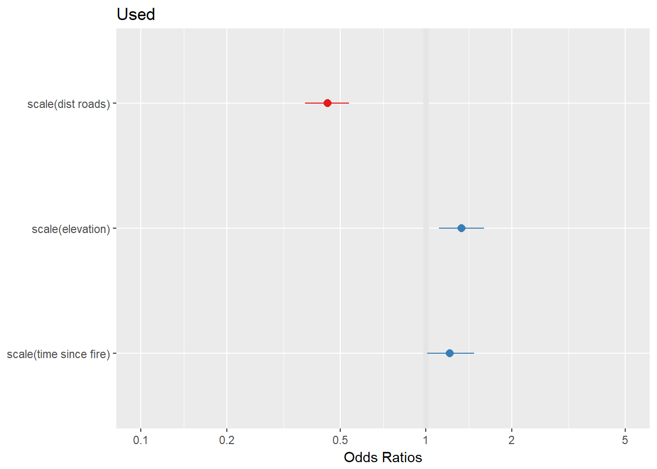
In our RSF that (incorrectly) uses an MCP to define availability, caribou appear to be selecting for older forests, and higher elevations, and appear to be preferring areas that are closer to roads (negative coefficient on distance = preference for closer distances).
Note that there is some correlation between higher elevations and distances to roads:
with(Data.rsf, plot(elevation, dist.roads, col = factor(Used)))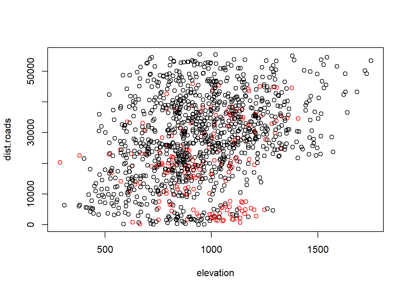
We might therefore consider a model that includes interactions:
RSF.fit2 <- glm(Used ~ scale(elevation) * scale(dist.roads) + scale(time.since.fire), data = Data.rsf, family = "binomial")
plot_model(RSF.fit2)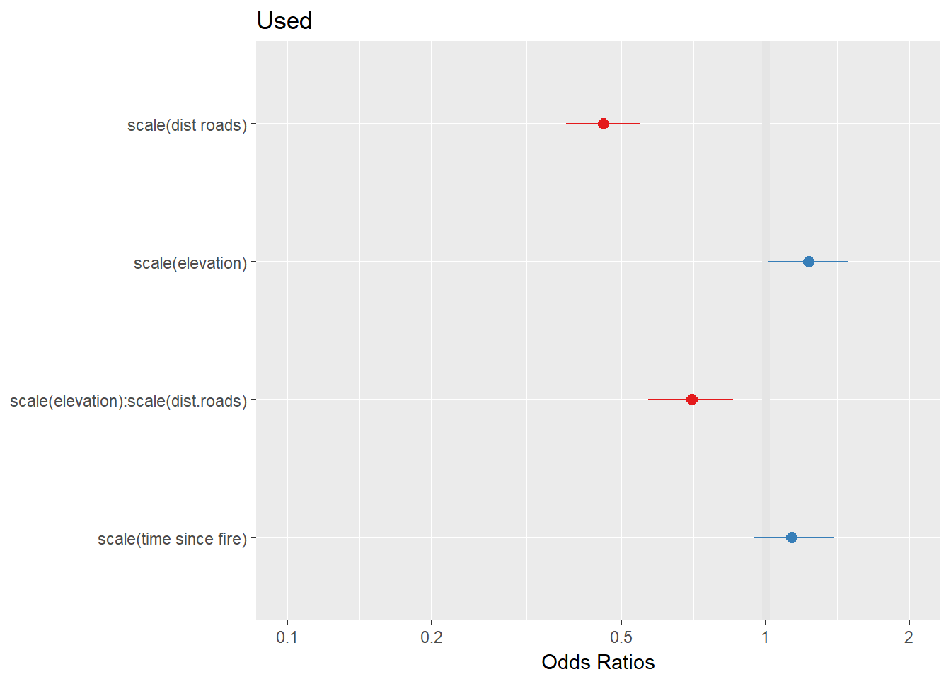
There’s a strong negative interaction, which suggests that at lower elevations, the preference for roads is weaker than at higher elevations. Is this a better model?
AIC(RSF.fit, RSF.fit2)## df AIC
## RSF.fit 4 1001.6336
## RSF.fit2 5 990.8531Yes, much better.
We might note that these deer are walking through intermediate elevations, and perhaps that preference is best modeled with, e.g., a second order polynomial. We can introduce a column of (scaled) squared elevation to the data:
Data.rsf$e2 <- Data.rsf$elevation^2
RSF.fit3 <-  glm(Used ~ (scale(elevation) + scale(e2)) * scale(dist.roads) + scale(time.since.fire), data = Data.rsf, family = "binomial")
plot_model(RSF.fit3)
AIC(RSF.fit, RSF.fit2, RSF.fit3)## df AIC
## RSF.fit 4 1001.6336
## RSF.fit2 5 990.8531
## RSF.fit3 7 986.9697An even better model, though. We might remove the (highly non-significant) e2 - dist.roads interaction. Note how I use the update function below:
RSF.fit4 <- update(RSF.fit3, formula = ~ . - scale(e2):scale(dist.roads))
AIC(RSF.fit, RSF.fit2, RSF.fit3, RSF.fit4)
## df AIC
## RSF.fit 4 1001.6336
## RSF.fit2 5 990.8531
## RSF.fit3 7 986.9697
## RSF.fit4 6 986.2218This sort of mucking around can go on forever (and the whole premise of this RSF is somewhat flawed), but for now, we’ll settle with this model and draw some RSF maps.
3.0.1 RSF prediction map
Make sure we have prediction scopes that match:
fmch.habitat.cropped <- crop(fmch.habitat, extent(caribou.sp))
fmch.rsf <- fmch.habitat.cropped[[1]]
Extract the appropriate vectors:
fmch.elevation.vector <- fmch.habitat.cropped[[1]]@data@values
fmch.fire.vector <- fmch.habitat.cropped[[2]]@data@values
fmch.dist.roads.vector <- fmch.habitat.cropped[[3]]@data@values
fmch.elevation2.vector <- (fmch.habitat.cropped[[1]]@data@values)^2
Predict.df <- data.frame(elevation = fmch.elevation.vector,
                         time.since.fire=fmch.fire.vector,
                         dist.roads=fmch.dist.roads.vector,
                         e2=fmch.elevation2.vector)
The key little function is predict (with newdata):
fmch.rsf@data@values <- predict(RSF.fit3, newdata = Predict.df)Plot the results:
plot(fmch.habitat[[1]], main = "elevation")
plot(fmch.habitat[[2]], main = "time since fire")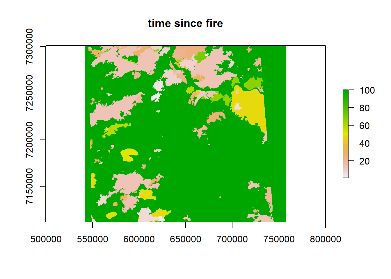
plot(fmch.habitat[[3]], main = "distance to roads")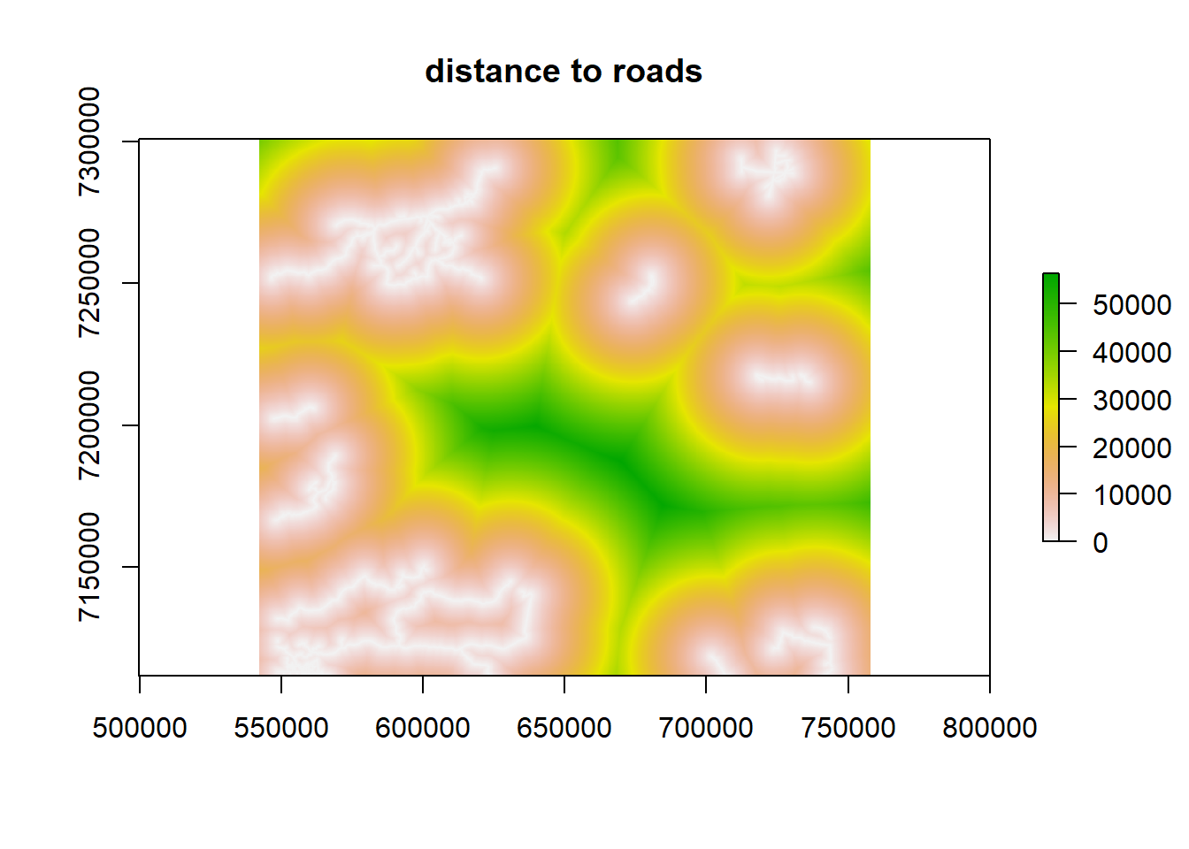
plot(fmch.rsf, main = "RSF", col = grey.colors(100, start = 0, end = 1))
points(caribou.sp, col = alpha("darkblue", 0.3), cex = 0.5)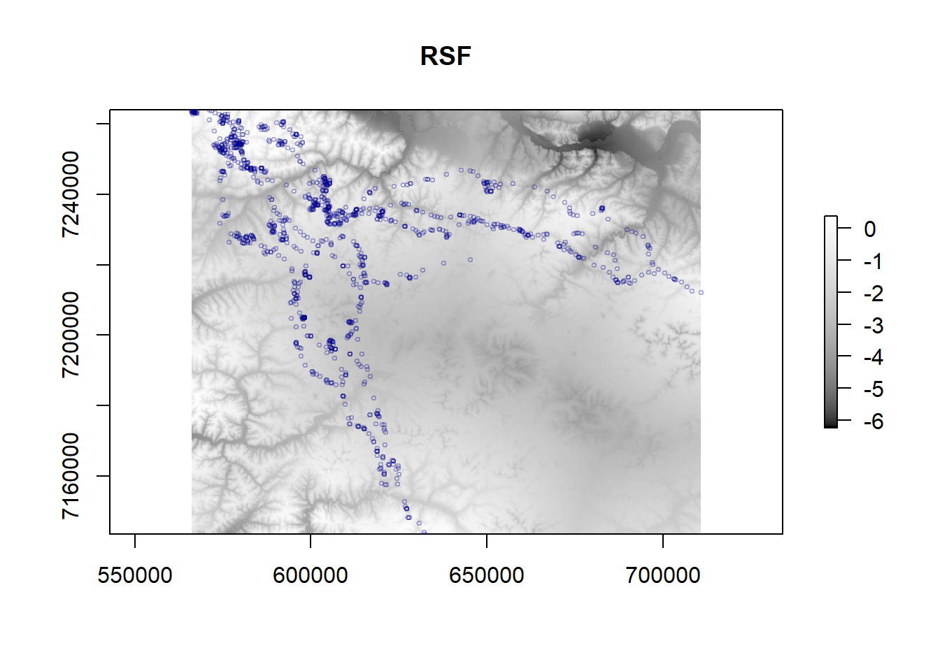
Again, don’t read too much into this result, because we violated a ton of assumptions, but at least now you have the basic workflow for conducting an RSF and visualizing the results!
4 Step-selection function
A step selection model is similar, but we compare for each “step” the environmental covariates of the selected step versus some sampling of possible steps.
We’ll be doing this with a relatively new package called amt.
require(amt)
require(sp)
4.1 Creating an amt track
For simplicity, we will start with just one animal. We need to specify coordinates, timestamp, and projection:
fa1403<- caribou.df %>%
  filter(id=="FA1403")

track1 <- mk_track(fa1403, x, y, time, crs=CRS("+proj=utm +zone=6 +ellps=WGS84 +datum=WGS84 +units=m +no_defs"))
summarize_sampling_rate(track1)
## # A tibble: 1 x 9
## min q1 median mean q3 max sd n unit
## <S3: table> <S3: > <S3: t> <S3: > <S3: > <S3: > <dbl> <int> <chr>
## 1 2.46666666666667 2.5 2.5 2.5 2.5 2.533~ 0.00556 307 hourWe see that the sampling rate is pretty consistent at one location every 2.5 hours, with little deviation.
If we want to look at the step length distribution:
steps.1 <- step_lengths(track1)
hist(steps.1, breaks = 30, main="Histogram of step lengths", xlab="Step lengths")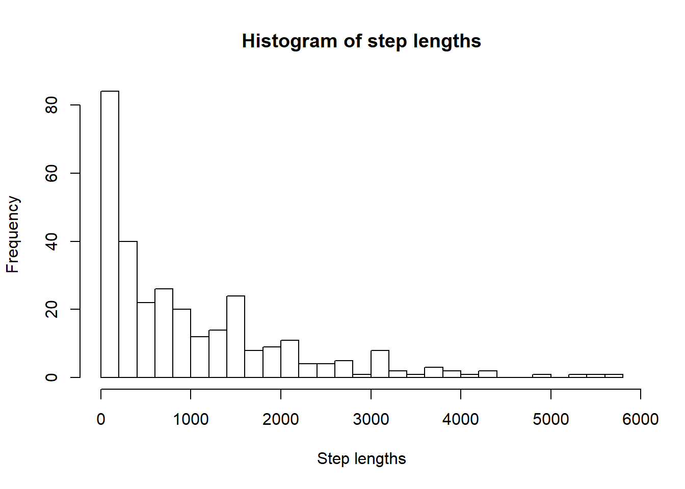
4.2 Create steps from points
Then we can create steps from the used points using the steps function:
true.steps1 <- steps(track1)
true.steps1## # A tibble: 307 x 9
## x1_ x2_ y1_ y2_ sl_ ta_ t1_
## <dbl> <dbl> <dbl> <dbl> <dbl> <dbl> <dttm>
## 1 610943. 610898. 7174743. 7174811. 80.3 NA 2017-08-10 00:00:00
## 2 610898. 610641. 7174811. 7176348. 1559. -23.8 2017-08-10 02:31:00
## 3 610641. 609672. 7176348. 7180358. 4125. 4.09 2017-08-10 05:00:00
## 4 609672. 608817. 7180358. 7186035. 5741. -5.01 2017-08-10 07:30:00
## 5 608817. 608971. 7186035. 7186773. 754. -20.4 2017-08-10 10:00:00
## 6 608971. 608659. 7186773. 7188044. 1309. 25.7 2017-08-10 12:30:00
## 7 608659. 608689. 7188044. 7190326. 2282. -14.6 2017-08-10 15:00:00
## 8 608689. 609760. 7190326. 7188796. 1868. -144. 2017-08-10 17:30:00
## 9 609760. 609760. 7188796. 7188793. 2.50 -12.8 2017-08-10 20:00:00
## 10 609760. 609759. 7188793. 7188797. 4.25 -176. 2017-08-10 22:30:00
## # ... with 297 more rows, and 2 more variables: t2_ <dttm>, dt_ <time>Creating 15 random (available) steps per used step:
true.random.steps1 <- random_steps(true.steps1, n = 15)Hopefully the figure below helps you visualize the “true” and “random” steps being created. “True” points or steps are often called “used” (these are in black), while “random” points or steps are often referred to as “available” or “psuedo-absences” (gray).
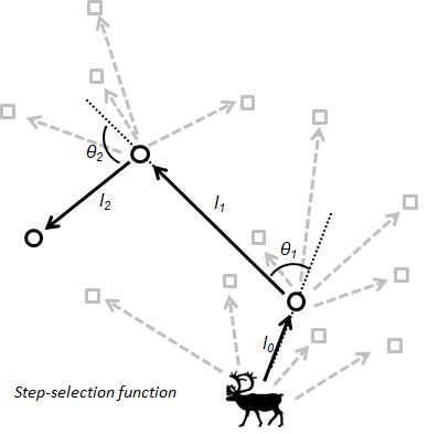
Now we extract the habitat covariates using the extract_covariates function in amt:
ssf1 <- true.random.steps1 %>% extract_covariates(fmch.habitat) Now we’re ready to fit a model.
We can run a conditional logistic regression comparing covariates at used points those at random points. Notice we are centering and scaling our covariates so they are easily comparable on the same scale.
ssf.1 <- clogit(case_ ~ strata(step_id_) + scale(elevation) + scale(time.since.fire) + scale(dist.roads) + scale(sl_), method = 'approximate', data = ssf1)plot_model(ssf.1, title="SSF Coefficients")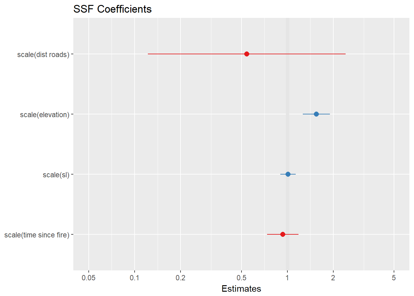
This individual is selecting for for higher elevations, but let’s try the same process below but with more than one caribou because just doing one animal isn’t very realistic.
5 SSF with multiple animals
The amt package doesn’t yet have documentation for running multiple animals, and the package author is planning to allow users to use the tidyverse of packages to do more of the data manipulation rather than write more custom functions. So we’ve created a nested data frame in dplyr (nesting by animal id) and created the track objects required by the package. The map function here is basically the same as lapply in base R, but it is in the package purrr in the tidyverse. We are applying the mk_track function in amt to each animal id (there are four), so we will get four “xyt tracks”
nested <-
caribou.df %>%
nest(-id) %>%
mutate(track = map(data, ~ mk_track(., x, y, time, crs= CRS("+proj=utm +zone=6 +ellps=WGS84 +datum=WGS84 +units=m +no_defs"))))
names(nested)## [1] "id" "data" "track"You can see that the nested object has columns for “data” and for “track”. Each of those columns is actually a list-column. “data” is a list of data frames, while “track” is a list of the track_xyt objects necessary for analysis in amt.
Similar to before, we are using the map function, applying the step_lengths function from amt to each of the track objects. After generating step lengths, let’s look at a histogram of them.
step.lengths <- unlist(map(nested$track, step_lengths))
hist(step.lengths, breaks = 20, main="Histogram of step lengths", xlab="Step lengths")
And the same process to look at summaries of the sampling rate for all individuals.
map(nested$track, summarize_sampling_rate)## [[1]]
## # A tibble: 1 x 9
## min q1 median mean q3 max sd n unit
## <S3: table> <S3: table> <S3: t> <S3:> <S3:> <S3:> <dbl> <int> <chr>
## 1 2.46666666666667 2.5 2.5 2.59~ 2.5 7.51~ 0.629 296 hour
##
## [[2]]
## # A tibble: 1 x 9
## min q1 median mean q3 max sd n unit
## <S3: table> <S3: > <S3: t> <S3: > <S3: > <S3: > <dbl> <int> <chr>
## 1 2.46666666666667 2.5 2.5 2.5 2.5 2.533~ 0.00646 307 hour
##
## [[3]]
## # A tibble: 1 x 9
##   min              q1     median  mean   q3     max         sd     n unit
##   <S3: table>      <S3: > <S3: t> <S3: > <S3: > <S3: >   <dbl> <int> <chr>
## 1 2.46666666666667 2.5    2.5     2.5    2.5    2.533~ 0.00556   307 hour
##
## [[4]]
## # A tibble: 1 x 9
## min q1 median mean q3 max sd n unit
## <S3: table> <S3: table> <S3: t> <S3:> <S3:> <S3:> <dbl> <int> <chr>
## 1 2.48333333333333 2.5 2.5 2.50~ 2.5 5 0.143 306 hourIf there were big time intervals between some successive locations, we might want to break the track up into bursts, and then we wouldn’t calculate distances and turn angles across bursts. Looks like the sampling rate is always around at 2.5 hours with not much deviation, so for simplicity, we won’t do this now.
5.1 Create steps from points
Generating steps from the points.
true.steps <- map(nested$track, steps)This object is a list of data frames (actually tibbles) that has coordinates of start and end points for each stetp, as well as step lengths and turning angles (in degrees, from -180 to 180).
Here’s the beginning of one tibble:
head(true.steps[[1]])## # A tibble: 6 x 9
## x1_ x2_ y1_ y2_ sl_ ta_ t1_
## * <dbl> <dbl> <dbl> <dbl> <dbl> <dbl> <dttm>
## 1 624774. 624633. 7162841. 7162385. 478. NA 2017-08-10 00:01:00
## 2 624633. 622227. 7162385. 7163133. 2520. -90.2 2017-08-10 02:30:00
## 3 622227. 622176. 7163133. 7163318. 192. -57.3 2017-08-10 07:31:00
## 4 622176. 621857. 7163318. 7163379. 325. 63.9 2017-08-10 10:00:00
## 5 621857. 620719. 7163379. 7160812. 2807. 76.8 2017-08-10 12:32:00
## 6 620719. 620778. 7160812. 7160625. 196. 41.2 2017-08-10 20:00:00
## # ... with 2 more variables: t2_ <dttm>, dt_ <time>5.2 Create random steps
Generating 10 random steps per used step.
true.random.steps <- map(true.steps, random_steps, n=10)Now that we’ve got the used and random steps, we’re just combining all the lists together so we can get a normal data frame for all four individuals. The .id="id" creates a new column with the id of the list so we can still separate data by animal.
all.steps <- bind_rows(true.random.steps, .id="id")
all.steps
## # A tibble: 13,332 x 12
## id step_id_ case_ x1_ y1_ x2_ y2_ t1_
## <chr> <int> <lgl> <dbl> <dbl> <dbl> <dbl> <dttm>
## 1 1 1 TRUE 624633. 7.16e6 6.22e5 7.16e6 2017-08-10 02:30:00
## 2 1 1 FALSE 624633. 7.16e6 6.26e5 7.17e6 2017-08-10 02:30:00
## 3 1 1 FALSE 624633. 7.16e6 6.24e5 7.16e6 2017-08-10 02:30:00
## 4 1 1 FALSE 624633. 7.16e6 6.25e5 7.16e6 2017-08-10 02:30:00
## 5 1 1 FALSE 624633. 7.16e6 6.25e5 7.16e6 2017-08-10 02:30:00
## 6 1 1 FALSE 624633. 7.16e6 6.28e5 7.17e6 2017-08-10 02:30:00
## 7 1 1 FALSE 624633. 7.16e6 6.24e5 7.16e6 2017-08-10 02:30:00
## 8 1 1 FALSE 624633. 7.16e6 6.23e5 7.16e6 2017-08-10 02:30:00
## 9 1 1 FALSE 624633. 7.16e6 6.21e5 7.16e6 2017-08-10 02:30:00
## 10 1 1 FALSE 624633. 7.16e6 6.25e5 7.16e6 2017-08-10 02:30:00
## # ... with 13,322 more rows, and 4 more variables: t2_ <dttm>, dt_ <time>,
## # sl_ <dbl>, ta_ <dbl>Here’s a distribution of turning angles for used steps only:
with(all.steps, hist(ta_[case_==T], breaks=20, main = "Histogram of turning angles", xlab="turning angle"))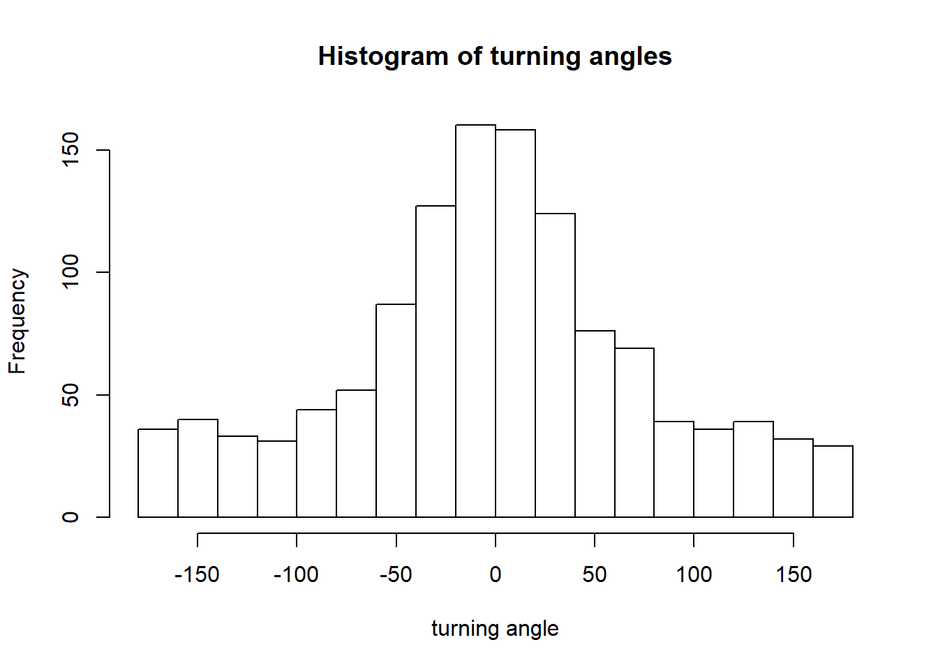
Unfortunately, by using the nested data frame, we’ve lost our projection information, which we need to extract points from the habitat covariate data. We’ll just convert to a SpatialPointsDataFrame so we can project it.
steps.sp <- all.steps
coordinates(steps.sp) <- ~x2_+y2_
proj4string(steps.sp) <- CRS("+proj=utm +zone=6 +ellps=WGS84 +datum=WGS84 +units=m +no_defs")
6 Extract habitat covariate data
Now we can extract the covariate data from the RasterStack…
covariates <- raster::extract(fmch.habitat, steps.sp)…and add the covariate data to our SpatialPointsDataFrame of used and random steps.
steps.sp$elevation <- covariates[,1]
steps.sp$tsf.years <- covariates[,2]
steps.sp$roads <- covariates[,3]
head(steps.sp)
## # A tibble: 6 x 13
## id step_id_ case_ x1_ y1_ t1_
## * <chr> <int> <lgl> <dbl> <dbl> <dttm>
## 1 1 1 TRUE 624633. 7162385. 2017-08-10 02:30:00
## 2 1 1 FALSE 624633. 7162385. 2017-08-10 02:30:00
## 3 1 1 FALSE 624633. 7162385. 2017-08-10 02:30:00
## 4 1 1 FALSE 624633. 7162385. 2017-08-10 02:30:00
## 5 1 1 FALSE 624633. 7162385. 2017-08-10 02:30:00
## 6 1 1 FALSE 624633. 7162385. 2017-08-10 02:30:00
## # ... with 7 more variables: t2_ <dttm>, dt_ <time>, sl_ <dbl>, ta_ <dbl>,
## # elevation <dbl>, tsf.years <dbl>, roads <dbl>Comparing elevation of used (true) vesus random (false) points
boxplot(elevation ~ case_, data = steps.sp, ylab="elevation")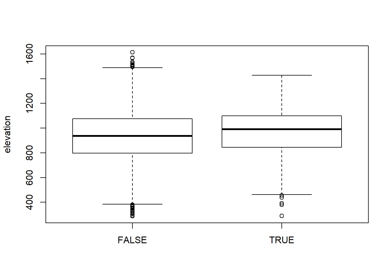
7 Run a model
Then we can run a conditional logistic regression comparing covariates at used points those at random points. Notice we are centering and scaling our covariates so they are easily comparable on the same scale.
SSF2 <- clogit(case_ ~ strata(step_id_) + scale(elevation) + scale(tsf.years) + scale(roads) + cluster(id) + scale(sl_), method = 'approximate', data = steps.sp)Looks like at the 2.5 hour time scale, animals are selecting for higher elevations, while time since fire and distance from road were not very important. Remember that this sampling scale is completely arbitrary.
And a similar plot as before:
plot_model(SSF2, title="SSF Coefficients")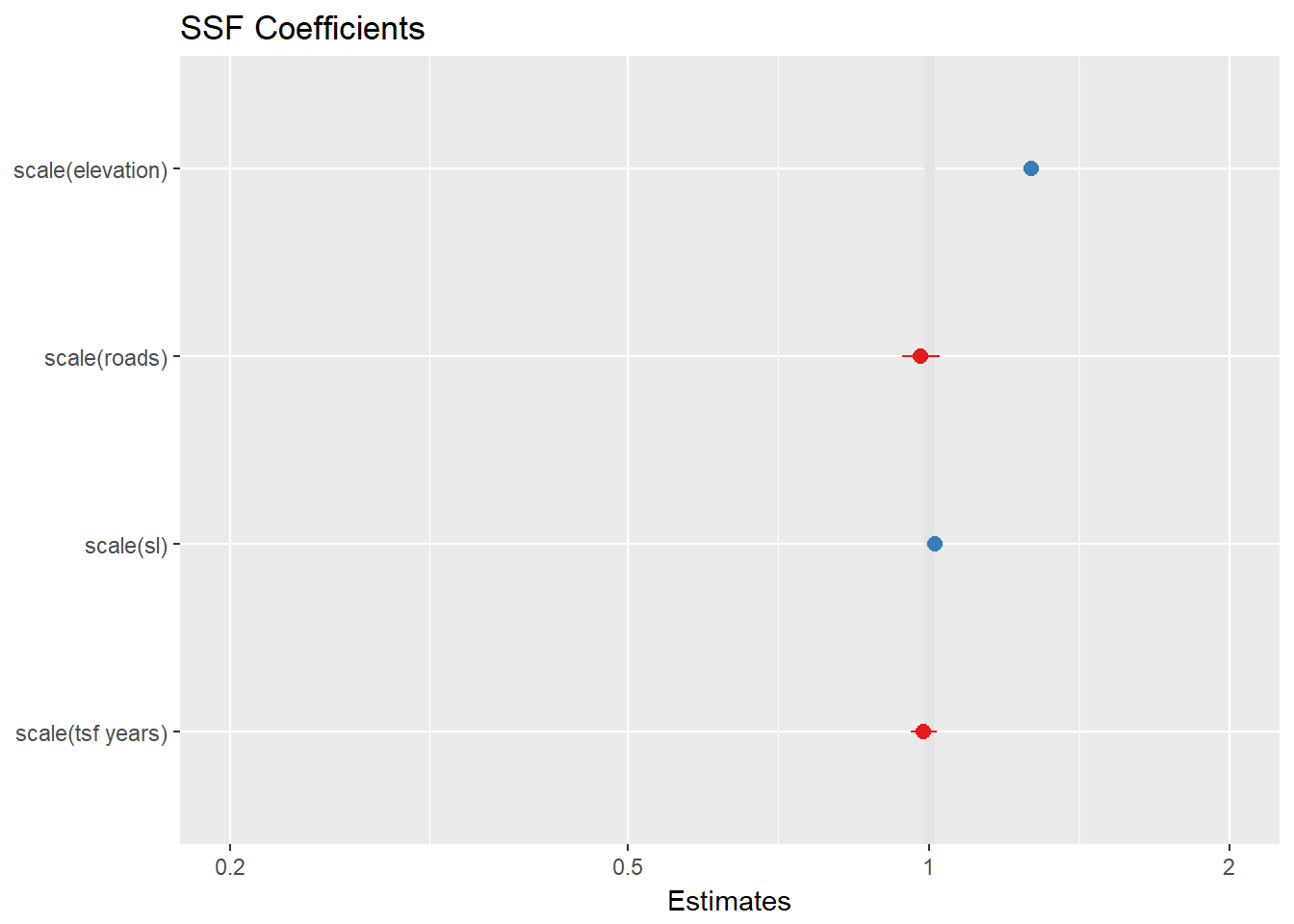
Mapping predictions of a conditional logistic regression model in space is difficult. We won’t attempt to do so here.