Processing Movement Data
Elie Gurarie and Eric Palm
1 Preamble
Processing data is the least loved and often most time consuming aspect of any data analysis. It is also unavoidable and extremely important. There are several tools - including some more recent R packages that greatly facilitate the processing of data.
Some broad guidelines of smart data processing include:
- compartamentalized - e.g. each step a function
- interactive - leverage visualization and interactive tools
- generalizable - to apply to multiple individuals
- replicable - important: NEVER overwrite the raw data!
- well-documented - so you don’t have to remember what you did
- forgettable! - so once its done you don’t need to think about it any more
2 Packages and functions
Several packages are particularly useful for data processing:
lubridate- manipulating time objectsrgdal- projecting coordinatesmapsandmapdata- quick and easy mapsdplyr- manipulating data frames and lists
Useful dplyr functions: mutate; group_by;select;summarize; filter
Sneaky R trick: For loading a lot of packages - makes a list:
pcks <- list('lubridate', 'ggmap', 'maptools', 'rgdal', 'maps', 'mapdata', 'move', 'dplyr', 'geosphere')and then “apply” the library function to the list:
sapply(pcks, library, character = TRUE)## [[1]]
## [1] "bindrcpp" "dplyr" "magrittr" "PBSmapping" "ggmap"
## [6] "ggplot2" "lubridate" "move" "rgdal" "raster"
## [11] "sp" "geosphere" "rmarkdown" "stats" "graphics"
## [16] "grDevices" "utils" "datasets" "methods" "base"
##
## [[2]]
## [1] "bindrcpp" "dplyr" "magrittr" "PBSmapping" "ggmap"
## [6] "ggplot2" "lubridate" "move" "rgdal" "raster"
## [11] "sp" "geosphere" "rmarkdown" "stats" "graphics"
## [16] "grDevices" "utils" "datasets" "methods" "base"
##
## [[3]]
## [1] "maptools" "bindrcpp" "dplyr" "magrittr" "PBSmapping"
## [6] "ggmap" "ggplot2" "lubridate" "move" "rgdal"
## [11] "raster" "sp" "geosphere" "rmarkdown" "stats"
## [16] "graphics" "grDevices" "utils" "datasets" "methods"
## [21] "base"
##
## [[4]]
## [1] "maptools" "bindrcpp" "dplyr" "magrittr" "PBSmapping"
## [6] "ggmap" "ggplot2" "lubridate" "move" "rgdal"
## [11] "raster" "sp" "geosphere" "rmarkdown" "stats"
## [16] "graphics" "grDevices" "utils" "datasets" "methods"
## [21] "base"
##
## [[5]]
## [1] "maps" "maptools" "bindrcpp" "dplyr" "magrittr"
## [6] "PBSmapping" "ggmap" "ggplot2" "lubridate" "move"
## [11] "rgdal" "raster" "sp" "geosphere" "rmarkdown"
## [16] "stats" "graphics" "grDevices" "utils" "datasets"
## [21] "methods" "base"
##
## [[6]]
## [1] "mapdata" "maps" "maptools" "bindrcpp" "dplyr"
## [6] "magrittr" "PBSmapping" "ggmap" "ggplot2" "lubridate"
## [11] "move" "rgdal" "raster" "sp" "geosphere"
## [16] "rmarkdown" "stats" "graphics" "grDevices" "utils"
## [21] "datasets" "methods" "base"
##
## [[7]]
## [1] "mapdata" "maps" "maptools" "bindrcpp" "dplyr"
## [6] "magrittr" "PBSmapping" "ggmap" "ggplot2" "lubridate"
## [11] "move" "rgdal" "raster" "sp" "geosphere"
## [16] "rmarkdown" "stats" "graphics" "grDevices" "utils"
## [21] "datasets" "methods" "base"
##
## [[8]]
## [1] "mapdata" "maps" "maptools" "bindrcpp" "dplyr"
## [6] "magrittr" "PBSmapping" "ggmap" "ggplot2" "lubridate"
## [11] "move" "rgdal" "raster" "sp" "geosphere"
## [16] "rmarkdown" "stats" "graphics" "grDevices" "utils"
## [21] "datasets" "methods" "base"
##
## [[9]]
## [1] "mapdata" "maps" "maptools" "bindrcpp" "dplyr"
## [6] "magrittr" "PBSmapping" "ggmap" "ggplot2" "lubridate"
## [11] "move" "rgdal" "raster" "sp" "geosphere"
## [16] "rmarkdown" "stats" "graphics" "grDevices" "utils"
## [21] "datasets" "methods" "base"3 Lesson Objectives
In this lesson, we will:
- Work with dates and times
- Learn how to work with projections of movement data
- Learn how to efficiently summarize movement data
4 Loading Data
Load the following caribou study from Movebank:
caribou <- getMovebankData(study="ABoVE: ADFG Fortymile Caribou (for TWS workshop)", login=login)Or - a useful habit to get into is saving your data as an R data file on your computer. This is done - simply - with save:
save(caribou, file = "./_data/caribou.raw.rda")Then, you can load itas needed. Note that saved R objects are more compact and much faster to load than, e.g., reading .csv’s (much less loading Movebank data off the internet), with the added advantage of retaining all the formatting and data type information.
You can then reload the data with the following command:
load("./_data/caribou.raw.rda")We’ll work with the data frame version:
caribou.df <- as(caribou, "data.frame")5 Data processing
5.1 Renaming columns
Movebank data comes with a set of (mostly) standard column names:
str(caribou.df)## 'data.frame': 1220 obs. of 28 variables:
## $ comments : Factor w/ 1 level "Fortymile Herd": 1 1 1 1 1 1 1 1 1 1 ...
## $ height_above_ellipsoid: num 871 881 1056 1061 1046 ...
## $ location_lat : num 64.6 64.6 64.6 64.6 64.6 ...
## $ location_long : num -144 -144 -144 -144 -144 ...
## $ timestamp : POSIXct, format: "2017-08-10 00:01:00" "2017-08-10 02:30:00" ...
## $ update_ts : Factor w/ 1 level "2018-03-19 14:00:01.038": 1 1 1 1 1 1 1 1 1 1 ...
## $ sensor_type_id : int 653 653 653 653 653 653 653 653 653 653 ...
## $ deployment_id : int 442813498 442813498 442813498 442813498 442813498 442813498 442813498 442813498 442813498 442813498 ...
## $ event_id : num 5.27e+09 5.27e+09 5.27e+09 5.27e+09 5.27e+09 ...
## $ location_long.1 : num -144 -144 -144 -144 -144 ...
## $ location_lat.1 : num 64.6 64.6 64.6 64.6 64.6 ...
## $ optional : logi TRUE TRUE TRUE TRUE TRUE TRUE ...
## $ sensor : Factor w/ 11 levels "Acceleration",..: 6 6 6 6 6 6 6 6 6 6 ...
## $ timestamps : POSIXct, format: "2017-08-10 00:01:00" "2017-08-10 02:30:00" ...
## $ trackId : Factor w/ 4 levels "FA17.09","FA1523",..: 1 1 1 1 1 1 1 1 1 1 ...
## $ individual_id : int 442813495 442813495 442813495 442813495 442813495 442813495 442813495 442813495 442813495 442813495 ...
## $ tag_id : int 442813490 442813490 442813490 442813490 442813490 442813490 442813490 442813490 442813490 442813490 ...
## $ id : int 442813498 442813498 442813498 442813498 442813498 442813498 442813498 442813498 442813498 442813498 ...
## $ comments.1 : Factor w/ 3 levels "","born in 2003",..: 1 1 1 1 1 1 1 1 1 1 ...
## $ death_comments : logi NA NA NA NA NA NA ...
## $ earliest_date_born : logi NA NA NA NA NA NA ...
## $ exact_date_of_birth : logi NA NA NA NA NA NA ...
## $ latest_date_born : logi NA NA NA NA NA NA ...
## $ local_identifier : Factor w/ 4 levels "FA1403","FA1523",..: 3 3 3 3 3 3 3 3 3 3 ...
## $ nick_name : logi NA NA NA NA NA NA ...
## $ ring_id : logi NA NA NA NA NA NA ...
## $ sex : Factor w/ 1 level "f": 1 1 1 1 1 1 1 1 1 1 ...
## $ taxon_canonical_name : Factor w/ 1 level "granti": 1 1 1 1 1 1 1 1 1 1 ...The nomenclature of these columns is important and unambiguous for movebank database purposes, but for the purposes of our own analyses the column names a bit long and unwieldly. Also - a lot of the data is not that interesting or important (though note the elevation sensor). We might simplify the data to a data frame that is more friendly:
caribou2 <- with(caribou.df, data.frame(id = trackId, lon = location_long, lat = location_lat, time = timestamp, elevation = height_above_ellipsoid))
head(caribou2)
## id lon lat time elevation
## 1 FA17.09 -144.3955 64.56772 2017-08-10 00:01:00 870.94
## 2 FA17.09 -144.3988 64.56368 2017-08-10 02:30:00 881.38
## 3 FA17.09 -144.4483 64.57127 2017-08-10 07:31:00 1056.01
## 4 FA17.09 -144.4493 64.57294 2017-08-10 10:00:00 1061.40
## 5 FA17.09 -144.4559 64.57360 2017-08-10 12:32:00 1046.44
## 6 FA17.09 -144.4817 64.55100 2017-08-10 20:00:00 910.77Note - it’s bad form to be renaming objects the same name as before, which is why I called this caribou2. It’s also not great form to have a whole bunch of caribou1-2-3’s, because that’s confusing. We’ll see later how to combine all the data processing into a single command.
5.2 Dates and Times
One of the scourges of movement data is dates and times, which are complicated and poorly stacked for a whole bunch of reasons related to inconsistent formatting, days and weeks and months not dividing nicely into years, etc.
The getMovebankData function (and, presumably, the Movebank database) nicely formats the times as POSIX - a standard universal data format for dates and times. If you are loading your data from a spreadsheet (e.g. via read.csv), you will have to convert the character strings into POSIX (otherwise they are loaded as factors). As an example, here is a sample of a text file containing African buffalo data:
buffalo <- read.csv("./_data/African_buffalo.csv", sep=",", header=TRUE)
str(buffalo)
## 'data.frame': 28410 obs. of 18 variables:
## $ event.id : int 10210419 10210423 10210428 10210434 10210456 10210458 10210483 10210535 10210544 10210558 ...
## $ visible : Factor w/ 1 level "true": 1 1 1 1 1 1 1 1 1 1 ...
## $ timestamp : Factor w/ 24489 levels "2005-02-17 05:05:00.000",..: 1 1 2 2 3 4 5 6 7 8 ...
## $ location.long : num 31.8 31.8 31.8 31.8 31.8 ...
## $ location.lat : num -24.5 -24.5 -24.5 -24.5 -24.5 ...
## $ behavioural.classification : int 0 0 0 0 0 0 0 0 0 0 ...
## $ comments : num 24.3 24.3 29.5 29.5 35.8 37.3 38.9 39.6 40 38.1 ...
## $ manually.marked.outlier : logi NA NA NA NA NA NA ...
## $ sensor.type : Factor w/ 1 level "gps": 1 1 1 1 1 1 1 1 1 1 ...
## $ individual.taxon.canonical.name: Factor w/ 1 level "Syncerus caffer": 1 1 1 1 1 1 1 1 1 1 ...
## $ tag.local.identifier : Factor w/ 6 levels "#1764820","#1764823",..: 1 1 1 1 1 1 1 1 1 1 ...
## $ individual.local.identifier : Factor w/ 6 levels "Cilla","Gabs",..: 5 5 5 5 5 5 5 5 5 5 ...
## $ study.name : Factor w/ 1 level "Kruger African Buffalo, GPS tracking, South Africa": 1 1 1 1 1 1 1 1 1 1 ...
## $ utm.easting : num 375051 375051 374851 374851 374527 ...
## $ utm.northing : num 7285726 7285726 7285502 7285502 7284538 ...
## $ utm.zone : Factor w/ 1 level "36S": 1 1 1 1 1 1 1 1 1 1 ...
## $ study.timezone : Factor w/ 1 level "South Africa Standard Time": 1 1 1 1 1 1 1 1 1 1 ...
## $ study.local.timestamp : Factor w/ 24489 levels "2005-02-17 07:05:00.000",..: 1 1 2 2 3 4 5 6 7 8 ...To convert the Date and Time into a POSIX object, you used to have to muck around with the as.POSIX commands R which could be quite clunky.
head(as.POSIXlt(paste(buffalo$timestamp), format = "%Y-%m-%d %H:%M:%S", tz = "UTC"))## [1] "2005-02-17 05:05:00 UTC" "2005-02-17 05:05:00 UTC"
## [3] "2005-02-17 06:08:00 UTC" "2005-02-17 06:08:00 UTC"
## [5] "2005-02-17 07:05:00 UTC" "2005-02-17 08:05:00 UTC"The lubridate package can generate these objects much more quickly, without specifying the formatting. The function ymd_hms below “intelligently” decifers the timestamp formatting of the data.
require(lubridate)
head(ymd_hms(buffalo$timestamp))
## [1] "2005-02-17 05:05:00 UTC" "2005-02-17 05:05:00 UTC"
## [3] "2005-02-17 06:08:00 UTC" "2005-02-17 06:08:00 UTC"
## [5] "2005-02-17 07:05:00 UTC" "2005-02-17 08:05:00 UTC"In this example, the time format was at least the (very sensible) YYYY-MM-DD. In the U.S> (and, it turns out, Canada) dates are often written down as MM/DD/YYYY (and, infuriatingly, always saved that way by Excel). For lubridate … no problem:
dates <- c("5/7/1976", "10-24:1979", "1.1.2000")
mdy(dates)
## [1] "1976-05-07" "1979-10-24" "2000-01-01"One other nice feature of lubridate is the ease of getting days of year, hour or days, etc. from data, e.g.:
hour(caribou2$time)[1:10]## [1] 0 2 7 10 12 20 22 1 3 6month(caribou2$time)[1:10]## [1] 8 8 8 8 8 8 8 8 8 8yday(caribou2$time)[1:10]## [1] 222 222 222 222 222 222 222 223 223 2235.3 Quick plot
require(ggplot2)
ggplot(caribou2, aes(x = lon, y = lat, col = id)) + geom_path()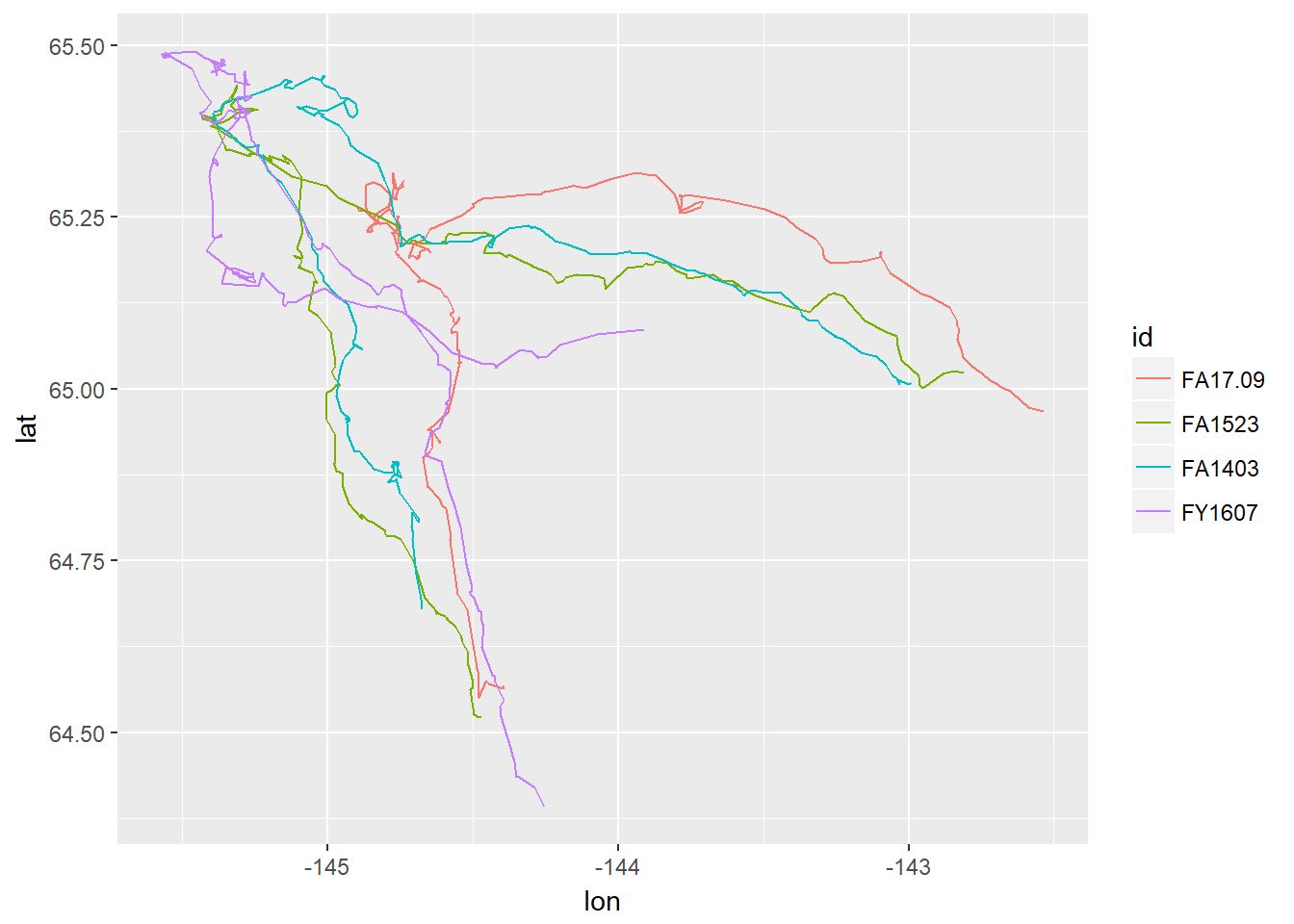
6 Projections
6.1 Latitudes, longitudes
It is nice to have Lat-Long data for seeing where your data are located in the world. But degrees latitude and longitude are not of consistent size, and movement statistics are best used in a consistent format, with “real” distances between points - whether in kilometers or meters.
6.1.1 … into UTM
One widely used type of projection for this purpose is “Universal transverse mercator” which will transform your data to meters north and east of one of 60 points at 6 degree intervals around the equator. One function that does this is convUL in PBSmapping. Its a bit awkward to use, as the data have to have columns names “X” and “Y” and have an “attribute” called “” “LL” so that it knows that its converting from a lat-long:
require(PBSmapping)
ll <- with(caribou2, data.frame(X = lon, Y = lat))
attributes(ll)$projection <- "LL"
xy.km <- convUL(ll, km=TRUE)
str(xy.km)
## 'data.frame': 1220 obs. of 2 variables:
## $ X: num 625 625 622 622 622 ...
## $ Y: num 7163 7162 7163 7163 7163 ...
## - attr(*, "projection")= chr "UTM"
## - attr(*, "zone")= num 6Note that the function determined that the best zone for these data would be zone 6. That is an easy variable to change. We can now say (roughly) that the total extent of the caribou movements was in kilometers:
diff(range(xy.km$X))## [1] 144.5833diff(range(xy.km$Y))## [1] 120.4752So over 120 km north-south, and 144 km east-west. You can add these transformed coordinates to the caribou data frame:
caribou3 <- data.frame(caribou2, x=xy.km$X*1000, y=xy.km$Y*1000)6.1.2 … using proj4
All projections (including) comprehensive projection standard is the PROJ4 system, which GIS users should be aware of. In particular when you are working with spatial files from other sources (e.g. habitat layers, bathymetry models), you need to make sure that your coordinates match up.
The original movebank loaded caribou object is an even more complex version of an SpatialPointsDataFrame object, itself a somewhat complex spatial data object:
is(caribou)## [1] "MoveStack" ".MoveTrackStack"
## [3] ".MoveGeneral" ".MoveTrack"
## [5] ".unUsedRecordsStack" "SpatialPointsDataFrame"
## [7] ".unUsedRecords" "SpatialPoints"
## [9] "Spatial" "SpatialVector"Its projection is:
caribou@proj4string## CRS arguments:
## +proj=longlat +ellps=WGS84 +datum=WGS84 +towgs84=0,0,0Which is the formal designation of Lat-Long on the WGS84 ellipsoid - the most common projection fro Lat-Long data.
We can reproject the caribou into any other projection, for example the UTM zone 6 projection (which you can look up here: http://www.spatialreference.org/ref/epsg/wgs-84-utm-zone-11n/) has the following proj4 code: +proj=utm +zone=6 +ellps=WGS84 +datum=WGS84 +units=m +no_defs
The function that re-projects these data is spTransform
projection <- CRS("+proj=utm +zone=6 +ellps=WGS84 +datum=WGS84 +units=m +no_defs")
caribou.utm <- spTransform(caribou, projection)
plot(caribou.utm)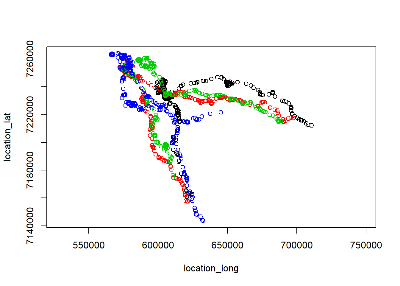
We can extract the x,y coordinates (as above) by converting to a data frame:
caribou.utm.df <- as(caribou.utm, "data.frame")
names(caribou.utm.df)
## [1] "comments" "height_above_ellipsoid"
## [3] "location_lat" "location_long"
## [5] "timestamp" "update_ts"
## [7] "sensor_type_id" "deployment_id"
## [9] "event_id" "location_long.1"
## [11] "location_lat.1" "optional"
## [13] "sensor" "timestamps"
## [15] "trackId" "individual_id"
## [17] "tag_id" "id"
## [19] "comments.1" "death_comments"
## [21] "earliest_date_born" "exact_date_of_birth"
## [23] "latest_date_born" "local_identifier"
## [25] "nick_name" "ring_id"
## [27] "sex" "taxon_canonical_name"Two new columns were added to the data frame: location_long.1 and location_lat.1 - there are the projected data.
xy.projected <- caribou.utm.df[,c("location_long.1", "location_lat.1")]A quick test to see if the two projections agree:
diff(range(xy.km[,1]))## [1] 144.5833diff(range(xy.projected[,1]))/1000## [1] 144.5833diff(range(xy.km[,2]))## [1] 120.4752diff(range(xy.projected[,2]))/1000## [1] 120.4752Excellent. So either method will work.
7 Summaries
dplyr is an excellent package for data manipulation. Here’s a helpful cheatsheet. dplyr uses the pipe operator, originally developed in the magrittr package which basically takes an object and passes it forward, so you can read your code left to right and limit the number of temporary files you create.
require(magrittr)
require(dplyr)
caribou3 %>%
  group_by(id) %>%
  summarize(
    n.obs = length(id),
        start = as.Date(min(time)),
        end = as.Date(max(time)),
        duration = max(time) - min(time),
        median.Dt = median(diff(time)),
        range.x = diff(range(x)),
        range.y = diff(range(y))
  )
## # A tibble: 4 x 8
## id n.obs start end duration median.Dt range.x range.y
## <fct> <int> <date> <date> <time> <time> <dbl> <dbl>
## 1 FA17.09 297 2017-08-10 2017-09-10 31.978472~ 2.5 112370. 86330.
## 2 FA1523 308 2017-08-10 2017-09-10 31.979166~ 2.5 124553. 101193.
## 3 FA1403 308 2017-08-10 2017-09-10 31.979166~ 2.5 114280. 86021.
## 4 FY1607 307 2017-08-10 2017-09-10 31.979166~ 2.5 79145. 120475.Visualize temporal extent of data:
ggplot(caribou3, aes(x = time, y = id)) + geom_path()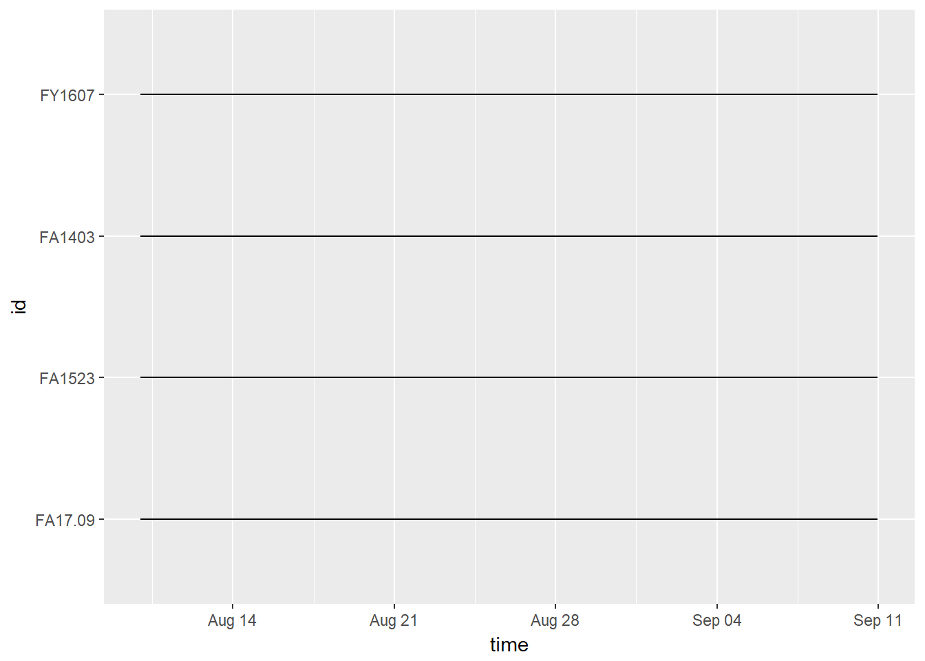
In this case, they’re all the same because we are just using a subset of data that starts August 10, 2017 and ends September 10, 2017.
The African Buffalo data we loaded earlier has some variation in temporal extent across marked animals:
ggplot(buffalo, aes(x = ymd_hms(timestamp), y = individual.local.identifier)) + geom_path()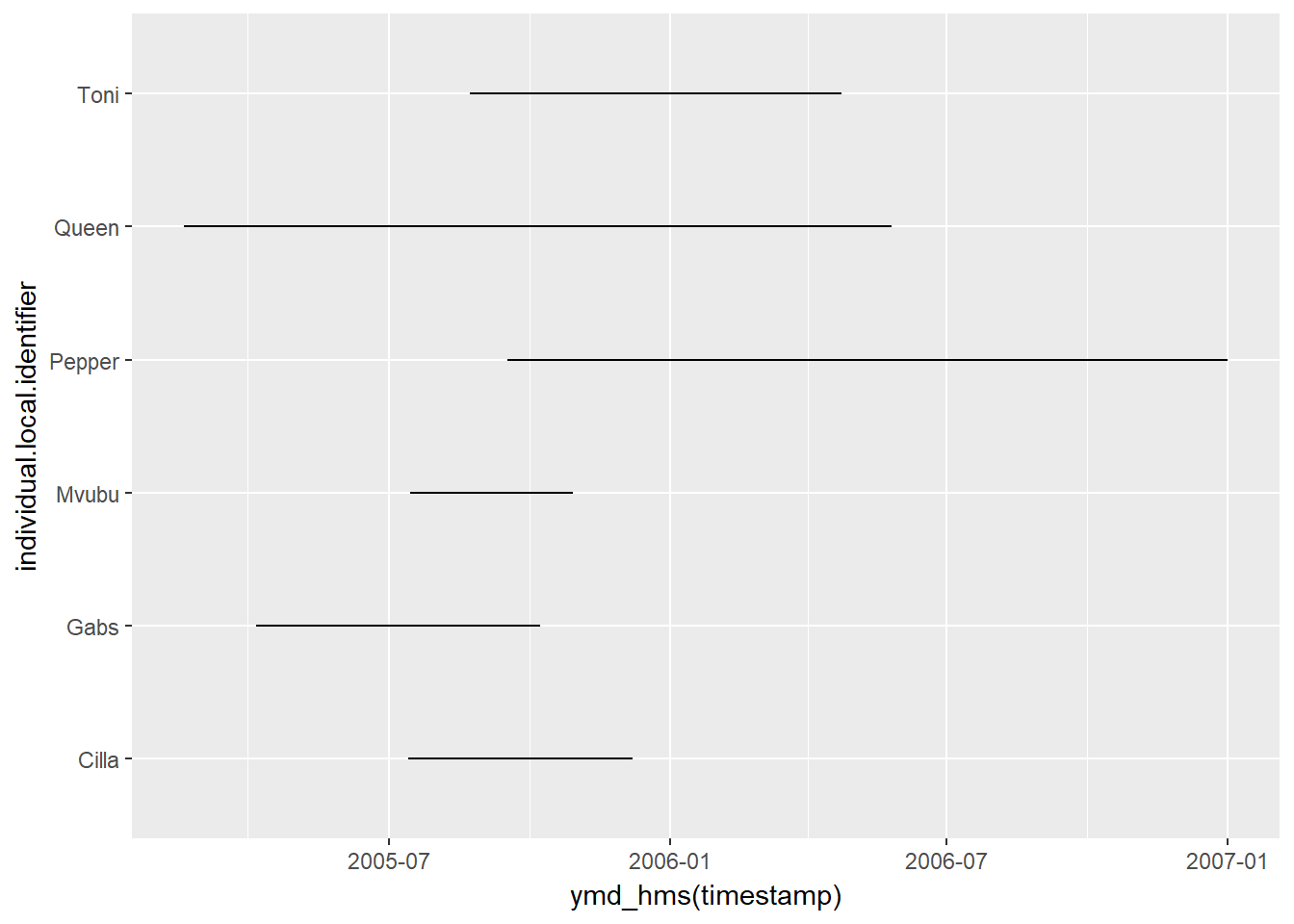
7.1 Aggregation
For some questions (e.g. major range shifts or migrations) we might not be interested in sub-daily processes. Also - the fact that the observation intervals are not entirely consistent can be annoying. With dplyr, it is easy to obtain, for example, a mean daily location. But first you need to obtain the day of each location.
caribou3$day.date <- as.Date(caribou3$time)caribou4 <- caribou3 %>%
group_by(id, day.date) %>%
summarize(
time = mean(time),
lon = mean(lon),
lat = mean(lat),
x = mean(x), y = mean(y),
elevation = mean(elevation)
)This is a much leaner (and therefore faster) data set:
dim(caribou3)## [1] 1220 8dim(caribou4)## [1] 128 8which, however, might lose a lot of the biology we are actually interested in.
8 One-step processing
As noted above, it’s bad form to be (a) renaming objects the same name as before, OR (b) also not great to have a whole bunch of caribou1-2-3’s, because that’s confusing. One way to really compact all of that code is to use the piping technique introduced above. You can explore examples and documentation, but in the meantime, compare the code below with the code above. After making a quick getUTM function (which converts lat long to UTM and adds x and y columns) we can combine all other steps sequentially into a single piped command:
load("./_data/caribou.raw.rda")
getUTM <- function(data){
    ll <- with(data, data.frame(X = lon, Y = lat))
    attributes(ll)$projection <- "LL"
    xy <- convUL(ll, km=TRUE)
    data.frame(data, x = xy$X, y = xy$Y)
}

caribou.daily.df <- caribou %>%
  as("data.frame") %>%
  dplyr::select(id = trackId,
         lon = location_long,
                 lat = location_lat,
                 time = timestamp,
                 elevation = height_above_ellipsoid) %>%
  mutate(day.date = as.Date(time)) %>%
  getUTM %>%
  group_by(id, day.date) %>%
  summarize(
    time = mean(time),
    lon = mean(lon),
    lat = mean(lat),
    x = mean(x),
    y = mean(y),
    elevation = mean(elevation)) %>%
as.data.frame()head(caribou.daily.df)## id day.date time lon lat x
## 1 FA17.09 2017-08-10 2017-08-10 10:43:25 -144.4443 64.56422 622.4520
## 2 FA17.09 2017-08-11 2017-08-11 11:38:00 -144.5056 64.61959 619.2791
## 3 FA17.09 2017-08-12 2017-08-12 14:31:00 -144.6126 64.82508 613.2968
## 4 FA17.09 2017-08-13 2017-08-13 12:44:00 -144.6422 64.91234 611.5279
## 5 FA17.09 2017-08-14 2017-08-14 10:53:15 -144.6342 64.94925 611.7512
## 6 FA17.09 2017-08-15 2017-08-15 13:45:22 -144.5486 65.04582 615.3788
## y elevation
## 1 7162.356 957.0343
## 2 7168.407 1069.9275
## 3 7191.098 926.1400
## 4 7200.764 1024.1633
## 5 7204.889 1294.6575
## 6 7215.799 1178.9413