Exploratory Analysis of Movement Data
Elie Gurarie and Eric Palm
1 Background
Before any modelling involving GPS movement data, it’s helpful to know how to calculate and summarize simple movement metrics that give you a better idea of what your animals are doing. This process may give rise to new questions or potential analysis ideas. You can also relate movements to different spatial features for which you have data.
1.1 Packages for movement summaries and spatial data
adehabitatLT- functions for movement trajectories; works in conjunction withadehabitatHR(home ranges),adehabitatHS(habitat selection), andadehabitatMA(habitat mapping)move- from Movebank team; uses objects of classmove,moveStackandmoveTrackctmm- not covered here, but a great package for continuous time movement models; can plot variograms (to view autocorrelation structure of data) and calculate autocorrelated kernel density estimate (AKDE) home ranges and Kriged occurrence distributions- We’ll also use the
dplyr,lubridate,ggplot2packages covered earlier sf(simple features) is a new package for handling spatial data that is a bit simpler thansp
1.2 Lab objectives
In this lab, we will:
- Calculate displacements, turn angles and speeds using a few different packages and functions
- Write and implement a function that adds these to a data frame
- Plot these movement metrics by individual and over time
- Annotate movement data using different types of spatial data, including rasters, polygons and polylines
pcks <- list("dplyr", "lubridate", "adehabitatLT", "ggplot2", "move") #, "sf")
sapply(pcks, require, char = TRUE)
## [1] TRUE TRUE TRUE TRUE TRUEFirst, load the caribou data frame and the (projected) caribou move object:
load("./_data/caribou.df.rda")
load("./_data/caribou.utm.rda")
2 Displacements, angles and speeds
One of the most basic movement statistics is simply displacement of each step (or step length). There are a few tools out there. For example if you convert your data to the native format of the adehabitatLT package (ltraj object) these are computed, and the move package has tools that compute them quickly. But there’s a “simple trick” to getting these variables very quickly; we refer you to this link for a detailed explanation.
2.1 Using our own functions
FA1403 <- subset(caribou.df, id == "FA1403")
Z <- FA1403$x + (0+1i) * FA1403$y
StepLength <- Mod(diff(Z))
Of course, step lengths depend on the GPX sampling interval, so we need to control for that and estimate “speed”:
dT <- as.numeric(diff(FA1403$time))
table(dT)
## dT
## 2.46666666666667 2.48333333333333 2.5 2.51666666666667
## 2 9 285 9
## 2.53333333333333
## 2We see that 285 of the 307 locations for this caribou were exactly 2.5 hours apart.
To calculate speed:
Speed <- StepLength/dTHere’s a summary of those speeds:
hist(Speed/1000, breaks = 50, col = "grey", xlab="km/hour", main="Speeds of caribou FA1403")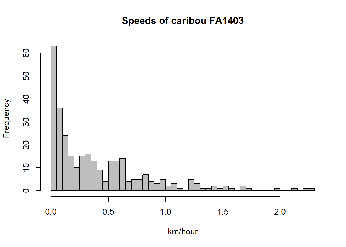
summary(Speed/1000)## Min. 1st Qu. Median Mean 3rd Qu. Max.
## 0.0003805 0.0723262 0.2719286 0.4029055 0.5949475 2.2965063Here’s a function that adds all those variables to the data frame:
computeDD <- function(data) {
    Z <- data$y + (0+1i) * data$y
    StepLength <- c(NA, Mod(diff(Z)))
    dT <- c(NA, as.numeric(diff(data$time)))
    Speed <- (StepLength/dT)/1000
    return(data.frame(data, StepLength, dT, Speed))
}
We can apply it to all four caribou:
caribou.df <- caribou.df %>%
  group_by(id) %>%
  computeDD
Now we can, for example, quickly see how movement rates vary across time using a simple box plot. Our caribou data are only from one month, so we’ll summarize speeds by hour, but you could summarize over weeks, months, day, etc.
boxplot((Speed) ~ hour(time), data = caribou.df,
    ylim = c(0, 4), ylab = "km/day", xlab="day of year", pch = 19, cex = 0.5, col = rgb(0, 0, 0, 0.5))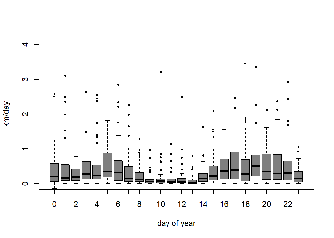
We could try to visualize this even better against hour of day across individuals with ggplot. Note: faceting allows us to compare individuals nicely, and the stat_smooth() feature draws a visual guide for the shifts. We’ll put speed on a log scale:
ggplot(subset(caribou.df, Speed>0), aes(x = hour(time), y = Speed)) +
  facet_grid(~id) + geom_point(alpha = 0.3) +
  stat_smooth() + scale_y_log10() +
  ylab("Speed (km/hr)") +  xlab("Hour of day")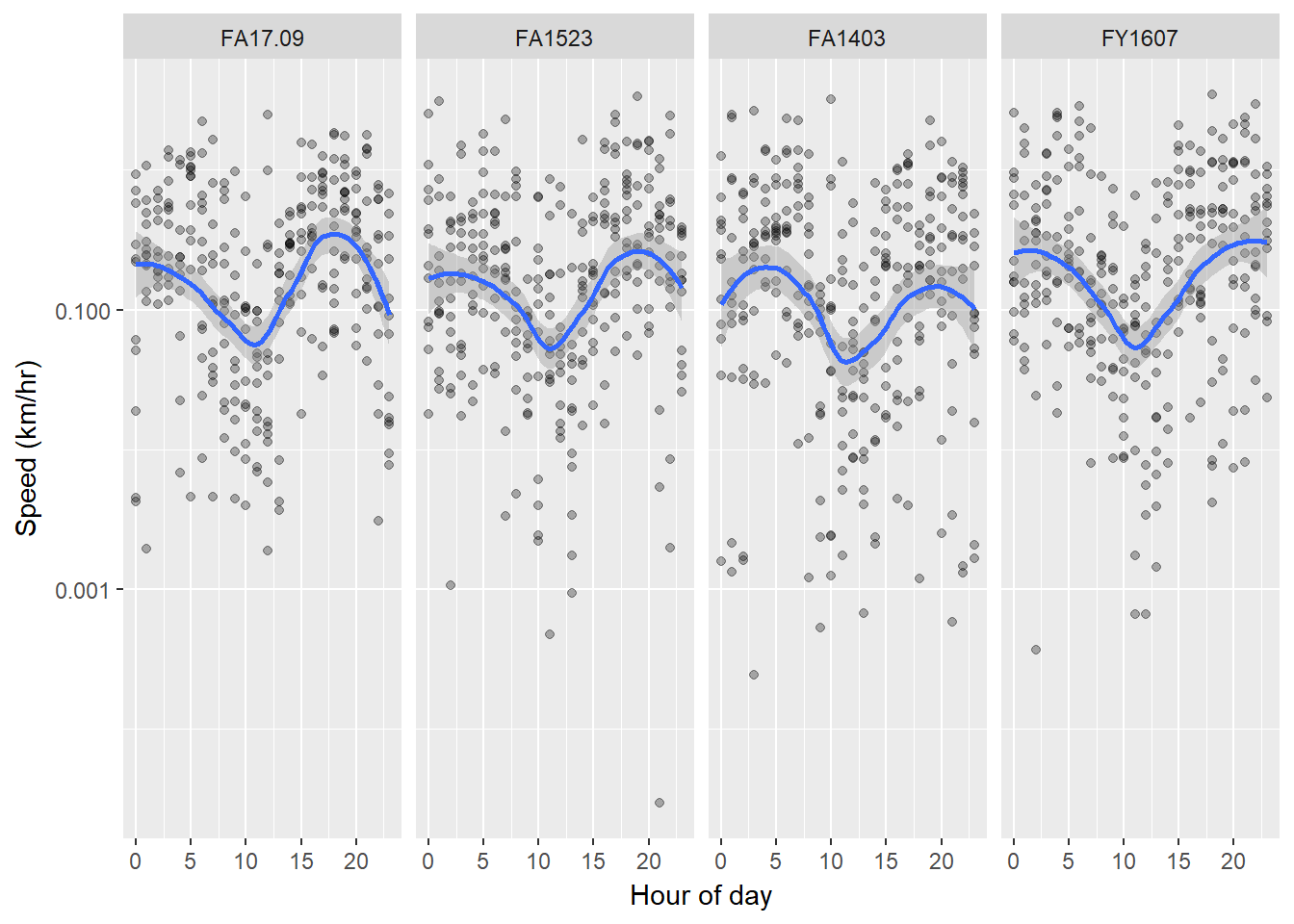
It appears that activity is lowest at mid day, and peaks at dusk and dawn …
2.1.0.1 ALERT!
…. but we have to be careful here, since the time of day is actually measured in UTC!
Here’s one way to convert:
caribou.df$time.ak <- caribou.df$time - dhours(9)
tz(caribou.df$time.ak) <- "US/Alaska"
ggplot(subset(caribou.df, Speed>0), aes(x = hour(time.ak), y = Speed)) +
facet_grid(~id) + geom_point(alpha = 0.3) + stat_smooth() +
scale_y_log10() + ylab("Speed (km/hr)") + xlab("Hour of day")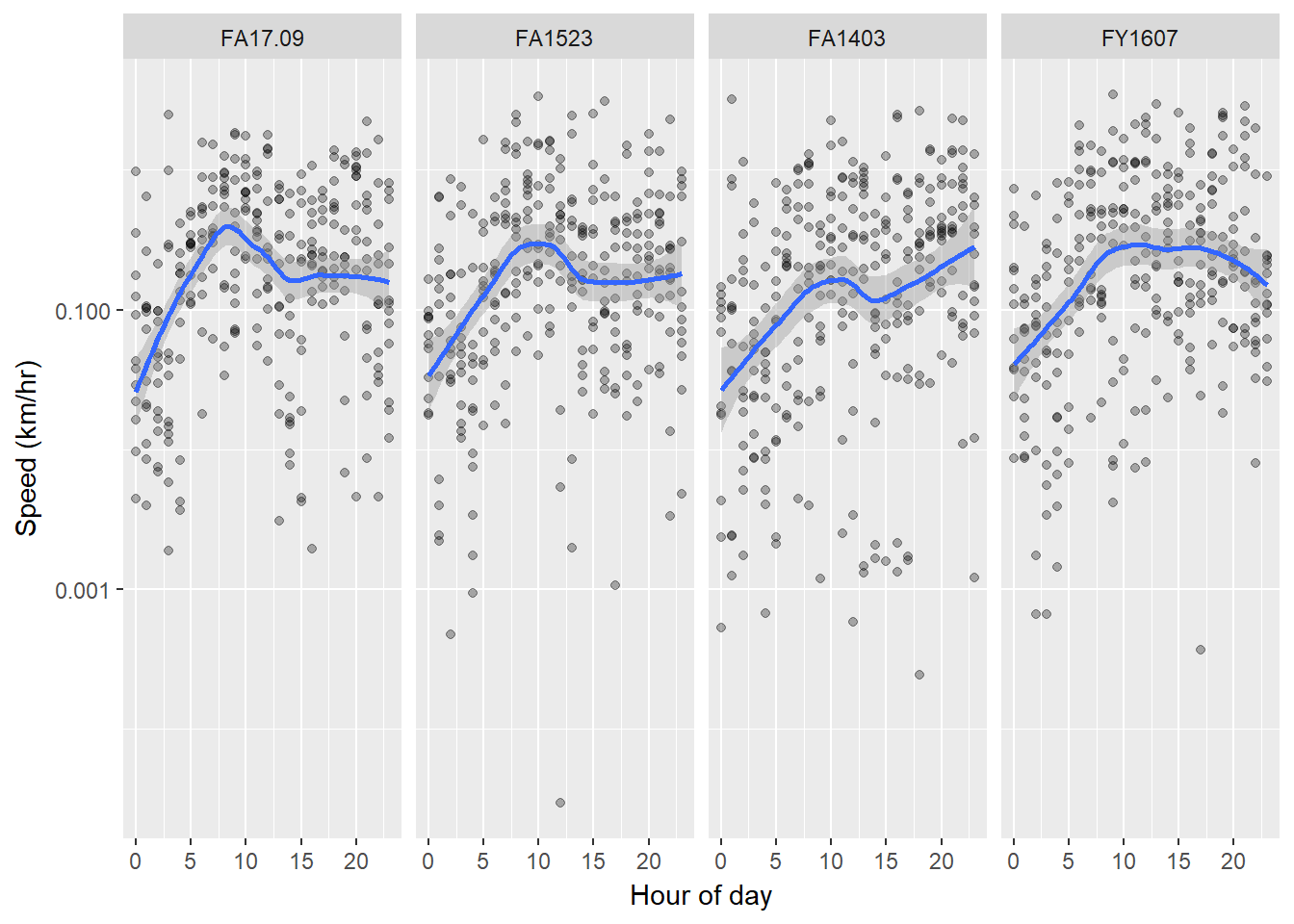
This gives a completely different (more correct) picture … of low activity at night, a peak at dawn and lower from mid-day on.
2.2 Using the move package
move has a distance function built in:
distances.move <- distance(caribou.utm)The result is a list, where each element is an individual caribou, and all the distances are components of those elements. This will give distances in meters.
One for sampling intervals:
timeLag.move <- timeLag(caribou.utm, units="hours")Again, the result is a list.
And one for speeds:
speeds.move <- move::speed(caribou.utm)For turn angles, move wants your data in lat/long which is what they are in when you first download from Movebank. We’ll quickly convert back to lat/long and then calculate turn angles:
caribou.move <- spTransform(caribou.utm, "+init=epsg:4326")
turn.angles.move <- turnAngleGc(caribou.move)
hist(unlist(turn.angles.move), main="Histogram of relative turn angles of four caribou", xlab="Relative turn angles", breaks=40)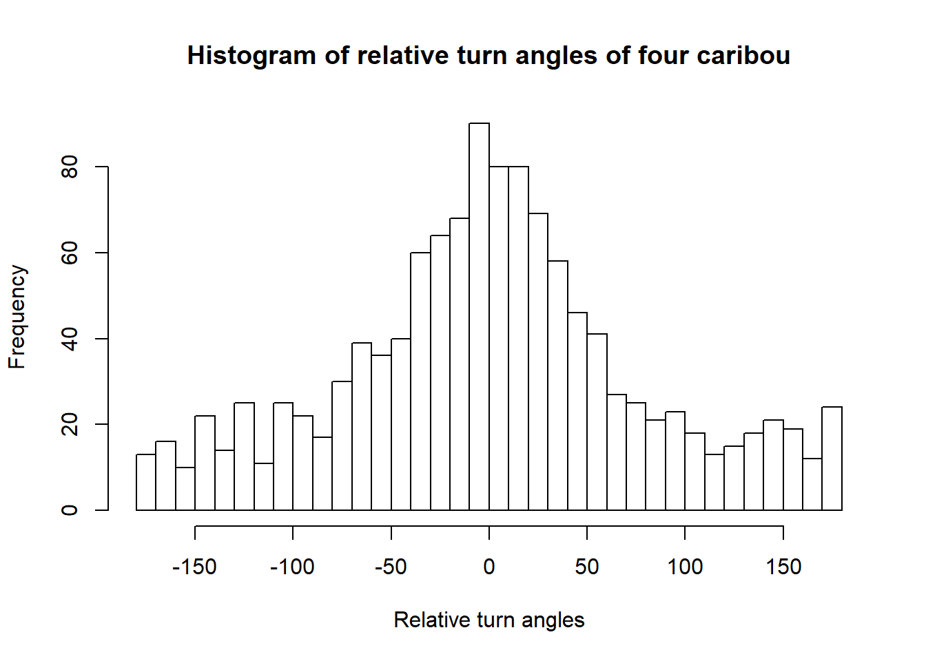
These are relative turn angles, with values between -180 and 180 degrees, meaning that they are calculated from the previous bearing of the animals. These are different than absolute turning angles, which are not related to the previous bearing.
2.3 Using adehabitatLT
adehabitatLT is for movement trajectories. At minimum, you need time, coordinates and id to create an ltraj object:
caribou.ltraj <- as.ltraj(xy = caribou.df[,c("x","y")], date = caribou.df$time, id = caribou.df$id)
caribou.ltraj
##
## *********** List of class ltraj ***********
##
## Type of the traject: Type II (time recorded)
## * Time zone: UTC *
## Irregular traject. Variable time lag between two locs
##
## Characteristics of the bursts:
## id burst nb.reloc NAs date.begin date.end
## 1 FA17.09 FA17.09 297 0 2017-08-10 00:01:00 2017-09-10 23:30:00
## 2 FA1523 FA1523 308 0 2017-08-10 00:00:00 2017-09-10 23:30:00
## 3 FA1403 FA1403 308 0 2017-08-10 00:00:00 2017-09-10 23:30:00
## 4 FY1607 FY1607 307 0 2017-08-10 00:00:00 2017-09-10 23:30:00
##
##
## infolocs provided. The following variables are available:
## [1] "pkey"This object is a list of data frames; one for each animal.
To view the data for the first caribou:
head(caribou.ltraj[[1]])## x y date dx dy dist
## 1 624773.5 7162841 2017-08-10 00:01:00 -140.48703 -456.38902 477.5223
## 2 624633.0 7162385 2017-08-10 02:30:00 -2405.86834 748.58438 2519.6391
## 3 622227.1 7163133 2017-08-10 07:31:00 -50.88552 184.67947 191.5616
## 4 622176.3 7163318 2017-08-10 10:00:00 -319.33958 60.56969 325.0330
## 5 621856.9 7163379 2017-08-10 12:32:00 -1137.59003 -2566.62796 2807.4348
## 6 620719.3 7160812 2017-08-10 20:00:00 58.29750 -186.88260 195.7644
## dt R2n abs.angle rel.angle
## 1 8940 0.0 -1.869415 NA
## 2 18060 228027.5 2.839939 -1.5738319
## 3 8940 6569303.8 1.839659 -1.0002796
## 4 9120 6973069.8 2.954148 1.1144884
## 5 26880 8795288.2 -1.988001 1.3410370
## 6 9000 20553883.8 -1.268415 0.7195855It automatically calculates the distance between successive locations (meters), relative and absolute turning angles (in radians), and time interval between successive locations (in seconds).
3 Spatial movement summaries
3.1 Annotating from a raster
Let’s compare the elevation by week of year (if you had a full year’s worth of data, grouping by seasons might be more meaningful). This is - in fact - very straightforward. We need only obtain the elevation at each point - a process sometimes referred to as “annotating” a movement dataset. In R, this is done from a raster with the extract function in the raster package. We can simply add a column to the caribou.df object, and then plot in ggplot:
load("./_data/fmch.habitat.rda")
elevation <- fmch.habitat[[1]]
caribou.df$elevation.dem <- raster::extract(elevation, caribou.df[, c("x", "y")])

ggplot(caribou.df, aes(as.factor(week(time)), elevation, col=id)) +
  geom_boxplot() +
  xlab("week of year")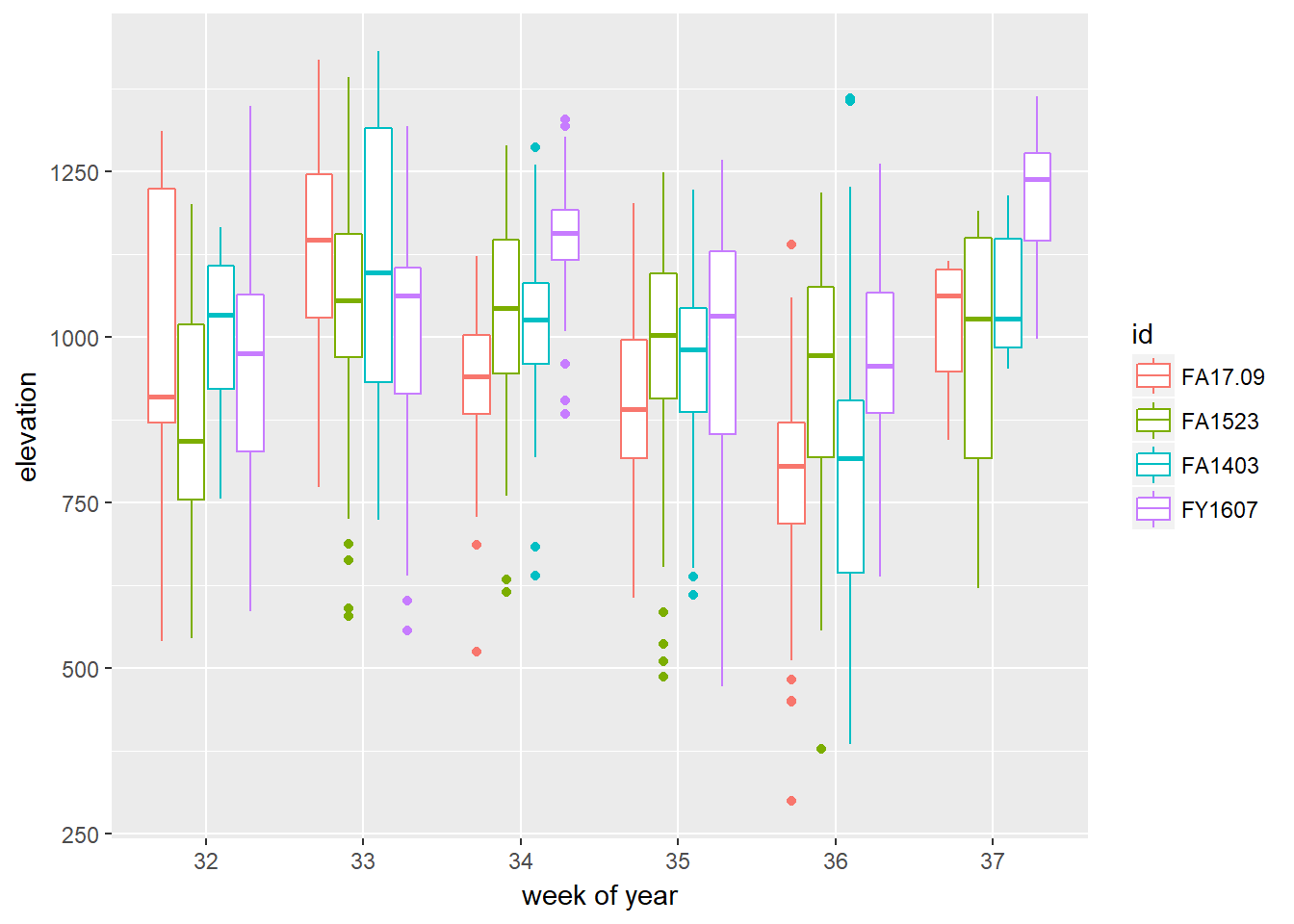
Since this dataset now has elevation data from a sensor on the collar itself and elevation data annotated from the DEM raster, we can quickly compare the two to see how well they agree:
with(caribou.df, plot(elevation, elevation.dem))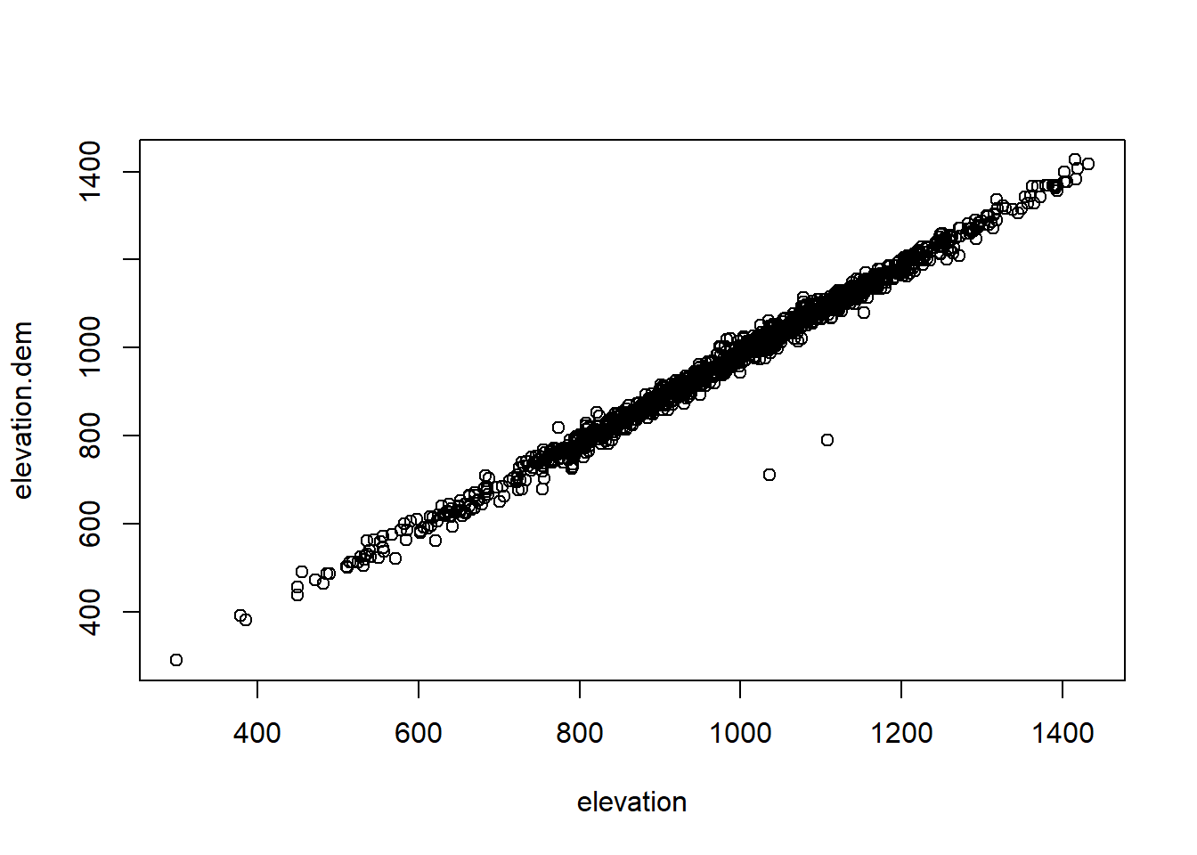
Pretty good! With the exception of those two rogue points…
3.2 Annotating from a polygon
We need to create an sf (simple features) object out of our caribou data to use with the sf package:
require(sf)
caribou.sf <- st_as_sf(caribou.df,
                        coords = c("x", "y"),
                        crs = "+proj=utm +zone=6 +ellps=WGS84 +datum=WGS84 +units=m +no_defs")
Bringing in our fires shapefile and transforming it to the same coordinate system of the caribou data:
fires <- st_read("./_data/fmch_fire_tws.shp")## Reading layer `fmch_fire_tws' from data source `c:\Users\elie\Box Sync\teaching\AlaskaWildlifeSociety\coursewebsite\_data\fmch_fire_tws.shp' using driver `ESRI Shapefile'
## Simple feature collection with 200 features and 51 fields
## geometry type: MULTIPOLYGON
## dimension: XYZ
## bbox: xmin: -146.0031 ymin: 63.99694 xmax: -141.9969 ymax: 66.00306
## epsg (SRID): 4269
## proj4string: +proj=longlat +datum=NAD83 +no_defsfires.utm <- st_transform(fires, "+proj=utm +zone=6 +ellps=WGS84 +datum=WGS84 +units=m +no_defs")Then we can do a spatial join between the two layers to see which locations are located within burns and which are not. We used dplyr::select to specify that we only want to add the FireYear column to the caribou.sf object, because otherwise it will add all the columns, which is more than we need. The ifelse statement just changes NAs to 0s (locations not in fire) and all others to 1.
caribou.sf <- st_join(caribou.sf, dplyr::select(fires.utm, FireYear)) # largest = TRUE
caribou.sf$fire <- as.factor(ifelse(is.na(caribou.sf$FireYear), 0, 1))
summary(caribou.sf$fire)
## 0 1
## 1124 97Only a small proportion of locations are located in fires.
Do caribou move more quickly through burned areas? Easy to visualize:
ggplot(caribou.sf, aes(id, Speed, col=fire)) +
  geom_boxplot()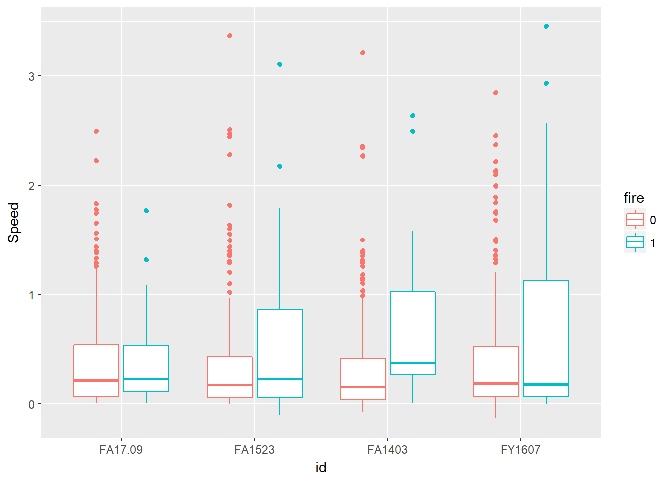
Looks like that might be true for some animals.
ggplot(caribou.sf, aes(id, elevation.dem, col=fire)) +
geom_boxplot()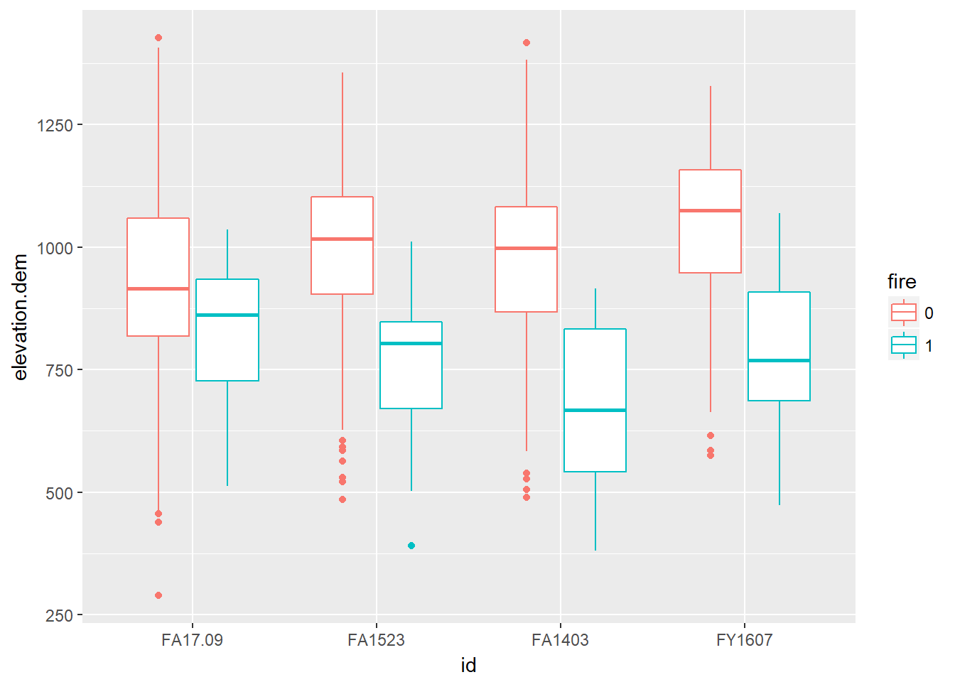 This shows that GPS locations in fires are at lower elevations, which is no surprise!
3.3 Distance from a polyline
If we have a polyline layer such as roads, we might want to calculate the minimum distance to any road for each point. Let’s bring in roads, transform it to the same projection as the caribou data, and use the st_distance function. The output is a matrix with distances between all combinations of points and roads. That’s more than what we want, so we’ll use the apply function to take the minimum value from each row of the matrix, which is the minimum distance between a point and any road.
roads <- st_read("./_data/fmch_roads_tws.shp")## Reading layer `fmch_roads_tws' from data source `c:\Users\elie\Box Sync\teaching\AlaskaWildlifeSociety\coursewebsite\_data\fmch_roads_tws.shp' using driver `ESRI Shapefile'
## Simple feature collection with 897 features and 11 fields
## geometry type: MULTILINESTRING
## dimension: XYZ
## bbox: xmin: -146.0031 ymin: 64.03747 xmax: -141.9969 ymax: 65.71606
## epsg (SRID): 4326
## proj4string: +proj=longlat +datum=WGS84 +no_defsroads.utm <- st_transform(roads, "+proj=utm +zone=6 +ellps=WGS84 +datum=WGS84 +units=m +no_defs")
dist.roads <- st_distance(caribou.sf, roads.utm)
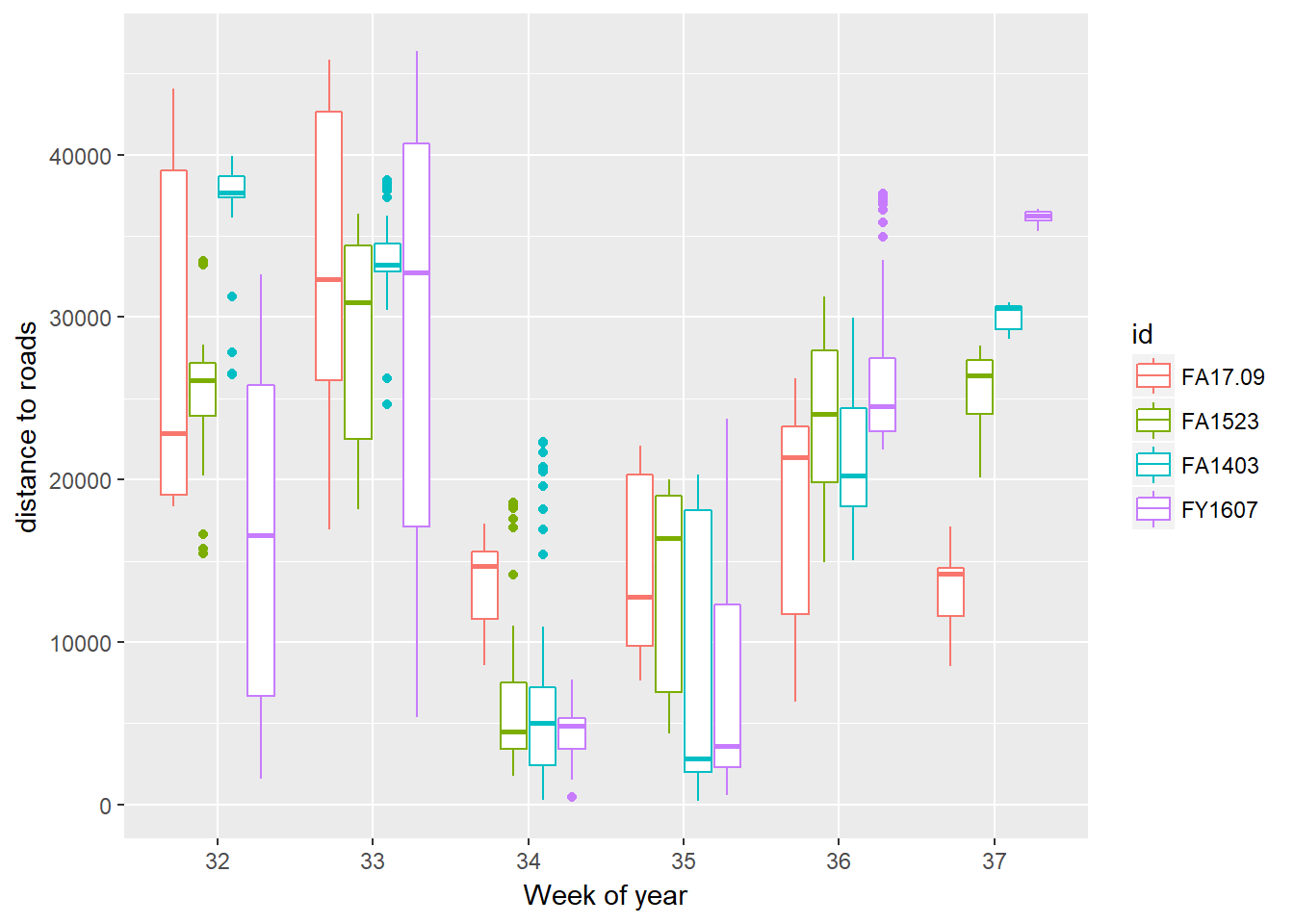
caribou.sf$dist.roads <- as.numeric(apply(dist.roads,1,min))A boxplot of distance to road by week of year, colored by individual caribou:
ggplot(caribou.sf, aes(as.factor(week(time)), dist.roads, col=id)) +
  geom_boxplot() +
  xlab("Week of year") +
  ylab("distance to roads")