Movebank
Elie Gurarie and Eric Palm
2018-03-29
1 Overview
Movebank is an online infrastructure to archive, share, manage, and analyze movement data.
Managed by the Max Planck Insitute, North Carolina Museum of Natural Sciences, and University of Konstanz.
1.1 Movebank goals
- Archive animal movement data for future use.
- Help scientists address questions by combining data sets from separate studies to test ecological or evolutionary ideas.
- Promote open access to animal movement data.
- 50% Studies NOT published
- ca. 9% movement data archived for open access
- Allow the public to explore the amazing animal movements recorded by animal trackers.
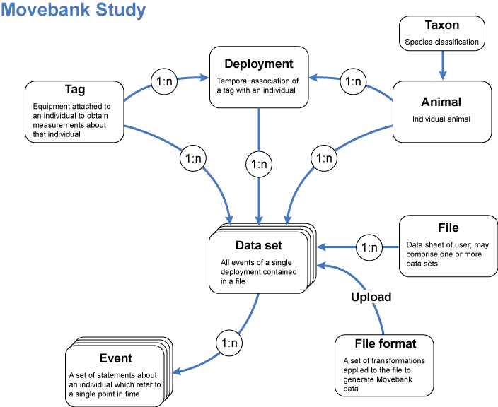
1.2 Movebank model (Kranstauber et al. 2011)

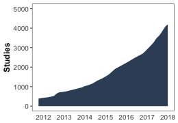
1.3 Movebank stats
As of January 2018:
- 17000 users (>5000 data owners)
- 756 taxa
- ca. 4182 studies
- Data archive: 88 datasets published

From Movebank
1.4 Alternative movement databases and repositories
- OBIS-SEAMAP (Ocean Biogeographic Information System Spatial Ecological Analysis of Megavertebrate Populations)
- ZoaTrack (Exploring and HR Estimates)
- UC-WRAM (Sweden, in progress)
1.5 Data Management
- Import data (GPS, Argos, bird rings, etc.), attributes, and other measurement from sensors (e.g. accelerometer). https://www.movebank.org/node/13
- Live data feeds (Argos PTT, GSM-GPS, Iridium GPS) are possible.
- Filter data based on duplicates, speed, or customized rules.
- Edit data (e.g. add/remove attributes, mark outliers, add behavior). Editing is faster in R (especially for larger datasets).
1.6 Data Sharing
- Same format for all data uploaded facilitating collaborative work.
- Data owners decide on sharing permissions.
- Data can be dowloaded as .csv, Excel, ESRI, etc. from Movebank website or using the package ‘move’ for R.
1.7 Data Analysis
- Data exploration through visualization
- Visualization tools linking movement and accelerometer data to environmental variables.
- Annotate tracking data with Env-DATA System. [Available environmental variables] (https://www.movebank.org/node/7471).
1.8 Data Archive
- Data is archived in the Movebank Data Repository for long-term use.
- It’s a way of formally published a movement dataset. Data will be reviewed, licensed for re-use, and citable.
1.9 Support
- support@movebank.org
- Sarah Davidson: sdavidson@orn.mpg.de
2 Using Movebank
If you don’t have an account yet, you can still see the tracking map, view studies and see some of the tracks. Some studies are not shown to the public and won’t show up in the tracking map.
If you want to upload/download data, you need to have an account. You can create one quickly and sign in.
You can go to the tracking data map and search for studies using the interactive map or by species. If you already have data, you can also go directly to the studies you have access to data because:
- you are the data manager
- you are a collaborator
- they are public
3 Uploading data from files
From the tracking data map, go to Upload (just above the query line).
If you are adding data to a study you already created, go to Add. Here you can add a new animal, new deployments for an existing animal or new tags.
If the data is part of a new study, you have to configurate a basic profile on your study first. Then you can go to Add and configurate details on animals, tags, and deployments.
To import data from files go to Upload > Import Data. You will need to indicate which column in your file corresponds to time, x, y, etc.
For real time data uploading, go to live-feed and select the type of sensor.
4 Accessing Movebank Data
4.1 … via Point-and-click
To download data from Movebank, go to the study site you are interested in and select Download. If you have permission to download already, you will only need to choose the data format you want. If you don’t have permission, contact the study manager. Make sure to introduce yourself and explain well the purpose of your work and why you need her/his data.
4.2 … directly into R
The following should help you directly access movebank.org via R, import movement data that you have permission to download, and convert these data into a data frame.
The key package to install is move
install.packages("move")
library(move)
require(lubridate)
Note that move relies on several very important (and powerful in their own right) packages for spatial analysis: sp, raster, rgdal and geosphere.
4.2.1 Step 1: A Login Object
Create a movebank.org login object, using your username and password
## login <- movebankLogin(username="xxxx", password="xxxx")4.2.2 Step 2: Loading a study
The first time you want to import movebank data, you have to make sure that you agree to the license agreement - via point-and-click on the movebank.org website. The steps for that are:
- In the tracking data map, search for the study you are interested in.
- Go to the study site.
- Select Download and it will show the agreement terms.
- Read them and agree.
Once you have accepted the license for that study, you can use the following simple line:
caribou <- getMovebankData(study="ABoVE: ADFG Fortymile Caribou (for TWS workshop)", login=login)Note: the name (with capitalization) of the study has to be entered exactly right.
There are some options that might be useful. For example, setting removeDuplicatedTimestamps=T is a quick to solve that problem.
This command can be somewhat slow (unclear why?), but in the end, it will have loaded the caribou data:
head(caribou)## comments height_above_ellipsoid location_lat location_long
## 617 Fortymile Herd 870.94 64.56772 -144.3955
## 618 Fortymile Herd 881.38 64.56368 -144.3988
## 619 Fortymile Herd 1056.01 64.57127 -144.4483
## 620 Fortymile Herd 1061.40 64.57294 -144.4493
## 621 Fortymile Herd 1046.44 64.57360 -144.4559
## 622 Fortymile Herd 910.77 64.55100 -144.4817
## timestamp update_ts sensor_type_id
## 617 2017-08-10 00:01:00 2018-03-19 14:00:01.038 653
## 618 2017-08-10 02:30:00 2018-03-19 14:00:01.038 653
## 619 2017-08-10 07:31:00 2018-03-19 14:00:01.038 653
## 620 2017-08-10 10:00:00 2018-03-19 14:00:01.038 653
## 621 2017-08-10 12:32:00 2018-03-19 14:00:01.038 653
## 622 2017-08-10 20:00:00 2018-03-19 14:00:01.038 653
## deployment_id event_id
## 617 442813498 5269591012
## 618 442813498 5269591013
## 619 442813498 5269591014
## 620 442813498 5269591015
## 621 442813498 5269591016
## 622 442813498 5269591017This is a MoveStack object, i.e. an S4 (formal class) with a bunch of “slots” containing information. If you have worked with the sp (spatial) package in R, objects of class move and MoveStack are just sp objects with a time component.
slotNames(caribou)## [1] "trackId" "timestamps"
## [3] "idData" "sensor"
## [5] "data" "coords.nrs"
## [7] "coords" "bbox"
## [9] "proj4string" "trackIdUnUsedRecords"
## [11] "timestampsUnUsedRecords" "sensorUnUsedRecords"
## [13] "dataUnUsedRecords" "dateCreation"
## [15] "study" "citation"
## [17] "license"Here are the counts of observations per caribou:
table(caribou@trackId)##
## FA17.09 FA1523 FA1403 FY1607
## 297 308 308 307Here is the bounding box (lower left and upper right coordinates):
caribou@bbox ## min max
## location_long -145.57223 -142.53494
## location_lat 64.39166 65.49057# or: bbox(caribou)etc.
4.3 Quick visualization
4.3.1 Basic plot
A basic plot of the caribou data:
plot(caribou)
S4 objects can be tricky to work with … for analysis R is much better suited to working with data frames and lists.
There are two ways to convert a move object to a data frame. The first is using the as.data.frame function:
caribou.df <- as.data.frame(caribou)
str(caribou.df)
## 'data.frame': 1220 obs. of 11 variables:
## $ comments : Factor w/ 1 level "Fortymile Herd": 1 1 1 1 1 1 1 1 1 1 ...
## $ height_above_ellipsoid: num 871 881 1056 1061 1046 ...
## $ location_lat : num 64.6 64.6 64.6 64.6 64.6 ...
## $ location_long : num -144 -144 -144 -144 -144 ...
## $ timestamp : POSIXct, format: "2017-08-10 00:01:00" "2017-08-10 02:30:00" ...
## $ update_ts : Factor w/ 1 level "2018-03-19 14:00:01.038": 1 1 1 1 1 1 1 1 1 1 ...
## $ sensor_type_id : int 653 653 653 653 653 653 653 653 653 653 ...
## $ deployment_id : int 442813498 442813498 442813498 442813498 442813498 442813498 442813498 442813498 442813498 442813498 ...
## $ event_id : num 5.27e+09 5.27e+09 5.27e+09 5.27e+09 5.27e+09 ...
## $ location_long.1 : num -144 -144 -144 -144 -144 ...
## $ location_lat.1 : num 64.6 64.6 64.6 64.6 64.6 ...This is okay, but we lose some of the animal data, such as sex, trackId, comments, etc.
Here’s a better option:
caribou.df <- as(caribou, "data.frame")
str(caribou.df)
## 'data.frame': 1220 obs. of 28 variables:
## $ comments : Factor w/ 1 level "Fortymile Herd": 1 1 1 1 1 1 1 1 1 1 ...
## $ height_above_ellipsoid: num 871 881 1056 1061 1046 ...
## $ location_lat : num 64.6 64.6 64.6 64.6 64.6 ...
## $ location_long : num -144 -144 -144 -144 -144 ...
## $ timestamp : POSIXct, format: "2017-08-10 00:01:00" "2017-08-10 02:30:00" ...
## $ update_ts : Factor w/ 1 level "2018-03-19 14:00:01.038": 1 1 1 1 1 1 1 1 1 1 ...
## $ sensor_type_id : int 653 653 653 653 653 653 653 653 653 653 ...
## $ deployment_id : int 442813498 442813498 442813498 442813498 442813498 442813498 442813498 442813498 442813498 442813498 ...
## $ event_id : num 5.27e+09 5.27e+09 5.27e+09 5.27e+09 5.27e+09 ...
## $ location_long.1 : num -144 -144 -144 -144 -144 ...
## $ location_lat.1 : num 64.6 64.6 64.6 64.6 64.6 ...
## $ optional : logi TRUE TRUE TRUE TRUE TRUE TRUE ...
## $ sensor : Factor w/ 11 levels "Acceleration",..: 6 6 6 6 6 6 6 6 6 6 ...
## $ timestamps : POSIXct, format: "2017-08-10 00:01:00" "2017-08-10 02:30:00" ...
## $ trackId : Factor w/ 4 levels "FA17.09","FA1523",..: 1 1 1 1 1 1 1 1 1 1 ...
## $ individual_id : int 442813495 442813495 442813495 442813495 442813495 442813495 442813495 442813495 442813495 442813495 ...
## $ tag_id : int 442813490 442813490 442813490 442813490 442813490 442813490 442813490 442813490 442813490 442813490 ...
## $ id : int 442813498 442813498 442813498 442813498 442813498 442813498 442813498 442813498 442813498 442813498 ...
## $ comments.1 : Factor w/ 3 levels "","born in 2003",..: 1 1 1 1 1 1 1 1 1 1 ...
## $ death_comments : logi NA NA NA NA NA NA ...
## $ earliest_date_born : logi NA NA NA NA NA NA ...
## $ exact_date_of_birth : logi NA NA NA NA NA NA ...
## $ latest_date_born : logi NA NA NA NA NA NA ...
## $ local_identifier : Factor w/ 4 levels "FA1403","FA1523",..: 3 3 3 3 3 3 3 3 3 3 ...
## $ nick_name : logi NA NA NA NA NA NA ...
## $ ring_id : logi NA NA NA NA NA NA ...
## $ sex : Factor w/ 1 level "f": 1 1 1 1 1 1 1 1 1 1 ...
## $ taxon_canonical_name : Factor w/ 1 level "granti": 1 1 1 1 1 1 1 1 1 1 ...Now we’ve retained all those attributes at the bottom.
4.3.2 ggmap
Here’s a quick ggmap of the caribou paths:
require(ggmap)Generate a basemap using the bounding boxes of the data. You can play with the zoom levels to get the extent you want.
basemap <- get_map(location = caribou@bbox, zoom = 8, maptype = "hybrid")Plot all the individuals:
ggmap(basemap) +
geom_path(data = caribou.df, mapping = aes(x = location_long, y = location_lat, col = trackId), alpha=.7, size=1) +
coord_map() + scale_colour_hue(l = 60) +
labs(x = "Longitude", y = "Latitude") + ggtitle("Fortymile caribou paths in late summer 2017") 
There are a few bells and whistles in this code to make it “prettier” that aren’t so important. But basically, you can see all the data at a glance, including some possible erroneous locations.