Introduction to dependent data: Time Series
BIOL709/BSCI339
Time Series Inferno:

Lasciate ogni speranza (di indipendenza), voi ch’entrate!
Translation: “Abandon all hope (of independence), ye who enter here!”
One slide summary of linear modeling
Simple: \[ Y_i = {\bf X} \beta + \epsilon_i \] \[ \epsilon_i \sim {\cal N}(0, \sigma^2) \] where \({\bf X}\) is the linear predictor and \(\epsilon_i\) are i.i.d.
Solved with: \(\hat{\beta} = ({\bf X}'{\bf X})^{-1}{\bf X}'y\).Generalized: \[ Y_i \sim \text{Distribution}(\mu) \] \[ g(\mu) = {\bf X} \beta \] where Distribution is exponential family and \(g(\mu)\) is the link function. Solved via iteratively reweighted least squares (IRLS).
Generalized Additive: \[Y_i \sim \text{Distribution}(\mu) \] \[ g(\mu_i) = {\bf X}_i \beta + \sum_{j} f_j(x_{ji}) \] where \({\bf X}_i\) is the \(i\)th row of X and \(f_j()\) is some smooth function of the \(j\)th covariate. Solved via penalized iteratively reweighted least squares (P-IRLS).
Note: In all of these cases \(i\) is unordered!
- \(Y_1, Y_2, Y_3 ... Y_n\) can be reshuffled: \(Y_5, Y_{42}, Y_2, Y_n ... Y_3\) with no impact on the results!
- In other words, all of the residuals: \(\epsilon_i = Y_i - \text{E}(Y_i)\) and \(\epsilon_j = Y_j - \text{E}(Y_j)\) are independent: \(\text{cov}{\epsilon_i, \epsilon_j} = 0\)
Basic Definitions
Stochastic process:
- Any process (data or realization of random model) that is structured by an index: \[ X_{t_{n}} = f(X_{t_1}, X_{t_2}, X_{t_3} ... X_{t_{n-1}})\] where \(f(\cdot)\) is a random process. The index can be time, spatial, location on DNA chain, etc.
Time-series:
- A stochastic process indexed by
- \(i \to t\): \(Y_1, Y_2, Y_3 ... Y_n\) becomes \(Y_{t_1}, Y_{t_2}, Y_{t_3} ... Y_{t_n}\)
Discrete-time time-series:
- Data collected at regular (Annual, Monthly, Daily, Hourly, etc.)~intervals.
- \(t\) usually denoted (and ordered) \(1, 2, 3, ... n\).
Continuous-time time-series:
-Data collected at arbitrary intervals: \(t_i \in \{T_{min}, T_{max}\}\).
Example of time series (and questions)
Question: Has the level of Lake Huron changed over 100 years?
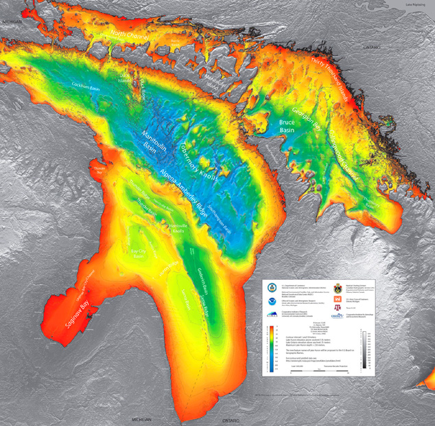
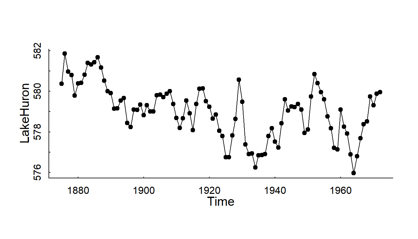
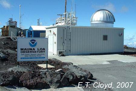
Question: Can we identify the trend / seasonal pattern / random fluctuations / make forecasts about CO2 emissions?

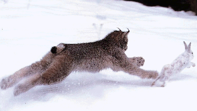
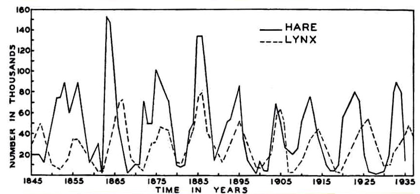
Question: What are the dynamics and relationships within and between lynx and hare numbers?[^1] [^1]: MacLulich Fluctuations in the numbers of varying hare, 1937
Question: How can we infer unobserved behavioral states from the movements of animals?

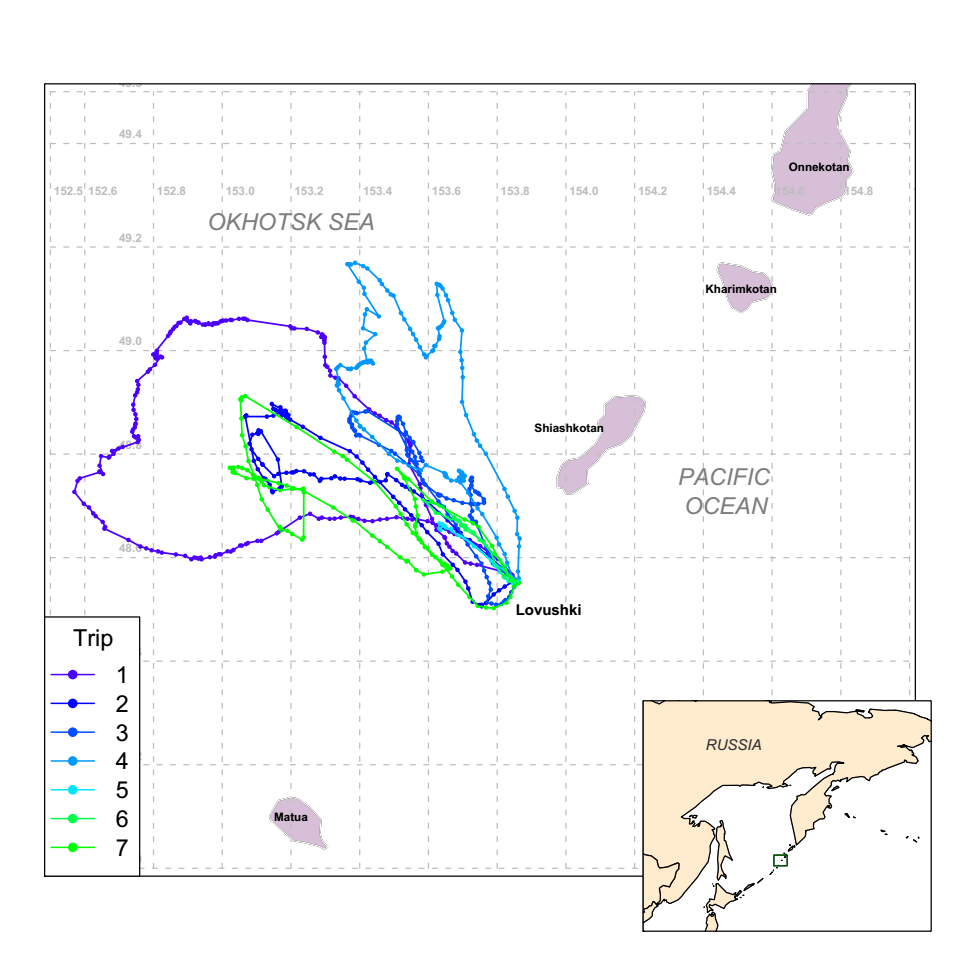
Note: Multidimensional state \(X\), continuous time \(T\)
Question: How can we quantify the time budgets and behaviors of a wolf?

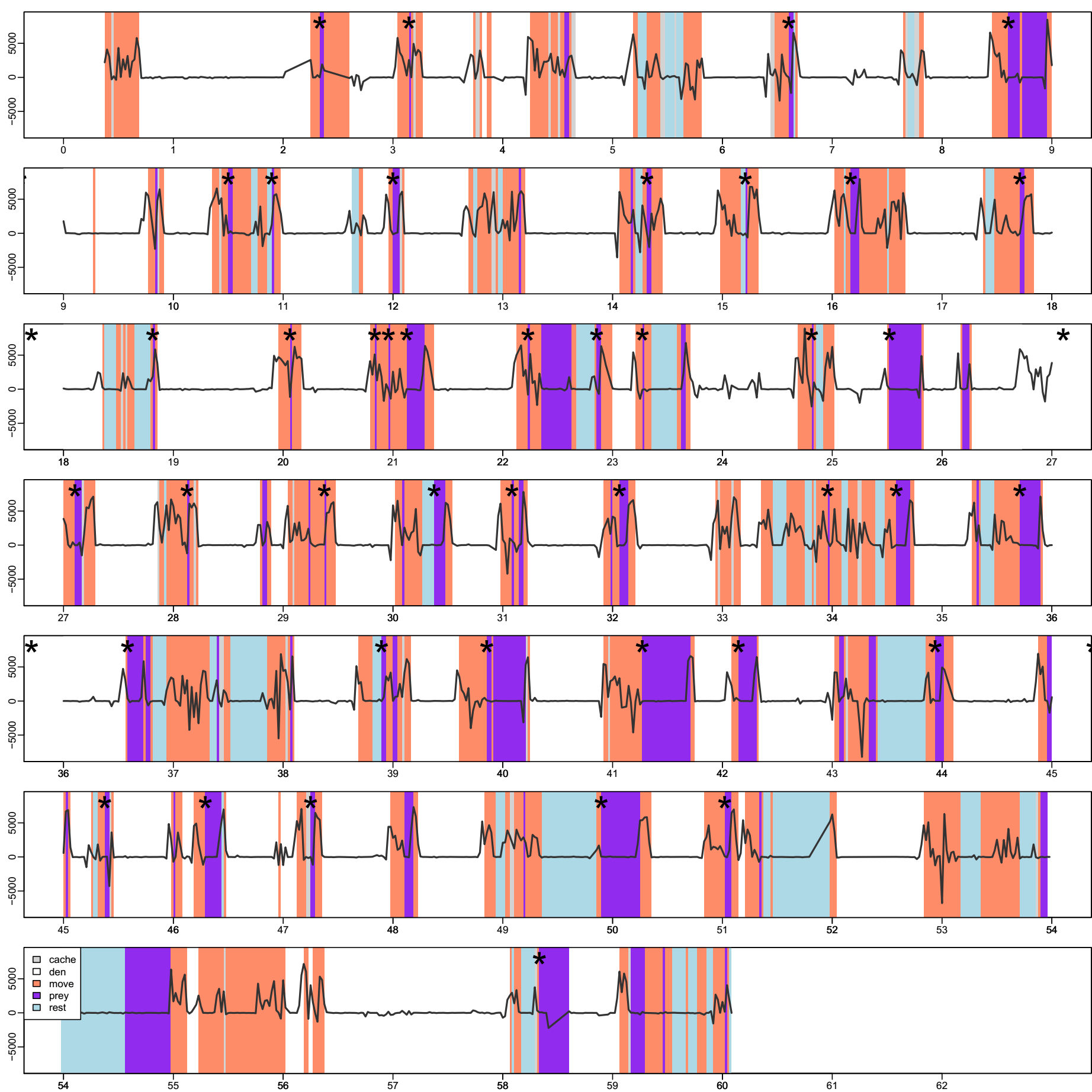
Note: Discrete states \(X\), continuous time \(T\)
Some objectives of time-series analysis
- Characterizing a random process
- Identifying trends, cycles, random structure
- Identifying and estimating the stochastic model for the time series
- Inference
- Accounting for lack of independence in linear modeling frameworks
- Avoiding FALSE INFERENCE!
- Learning something important the autocorrelation structure
- Forecasting
Concept 1: Autocorrelation
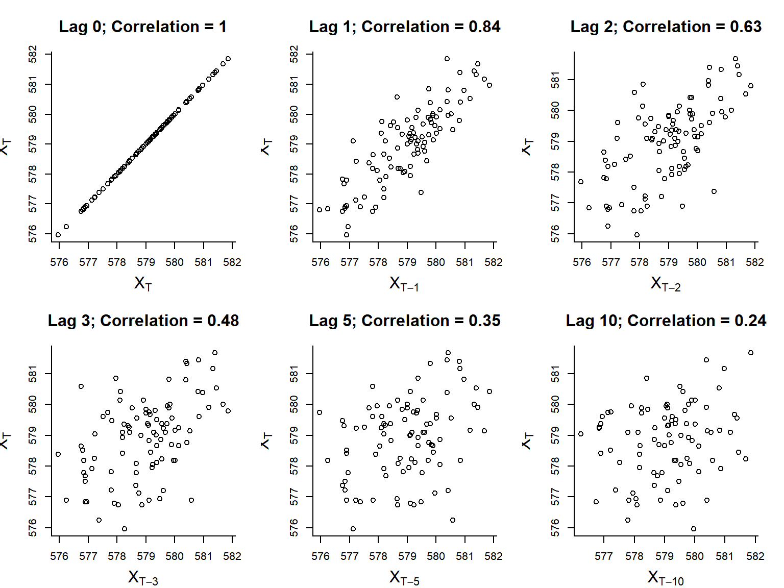
- Autocovariance function: \(\gamma(h) = \text{cov}[X_t, X_{t-h}]\)
- Autocorrelation function (acf): \(\rho(h) = \text{cor}[X_t, X_{t+h}]\)
Estimates
- Sample mean: \[\overline{X} = {1 \over n}\sum_{t=1}^n X_t\]
- Sample autocovariance: \[\widehat{\gamma}(h) = {1 \over n} \sum_{t=1}^{n-|h|} (X_{t+|h|} - \overline{X})(X_t - \overline{X})\]
- Sample autocorrelation: \[\widehat{\rho}(h) = {\widehat{\gamma}(h) \over \widehat{\gamma}(0)}\]
Sample autocorrelation
in R:
acf(X)
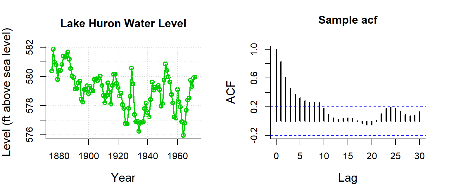
Lake Huron
Gives an immediate sense of the significance / shape of autocorrelation
White Noise
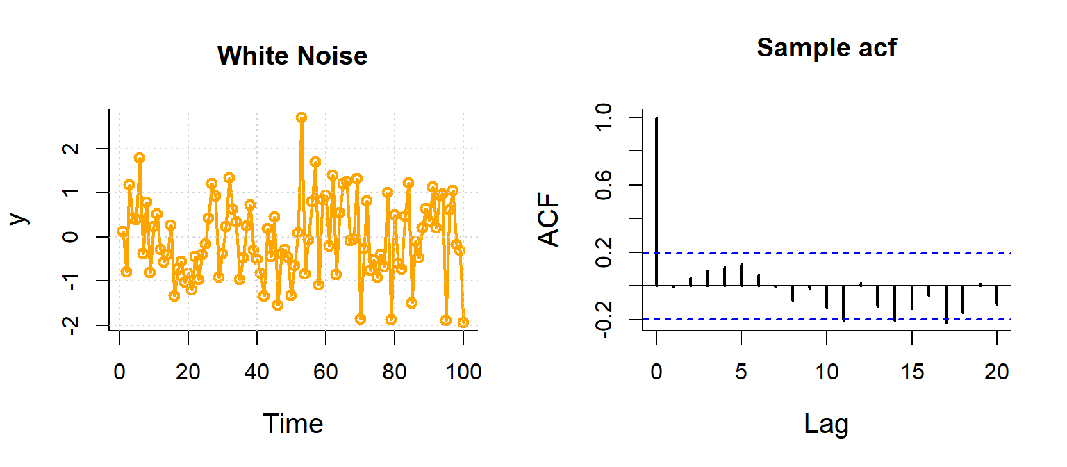
Note, blue dashed line is \(1.96 \over \sqrt{n}\), because expected sample autocorrelation for white noise is \(\sim {\cal N}(0,1/n)\)
Lynx
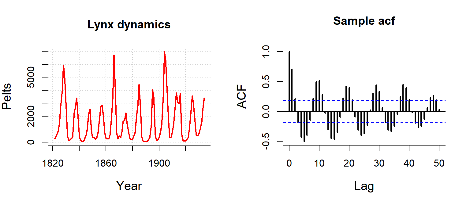
ACF provides instant feel for periodic patterns.
CO2
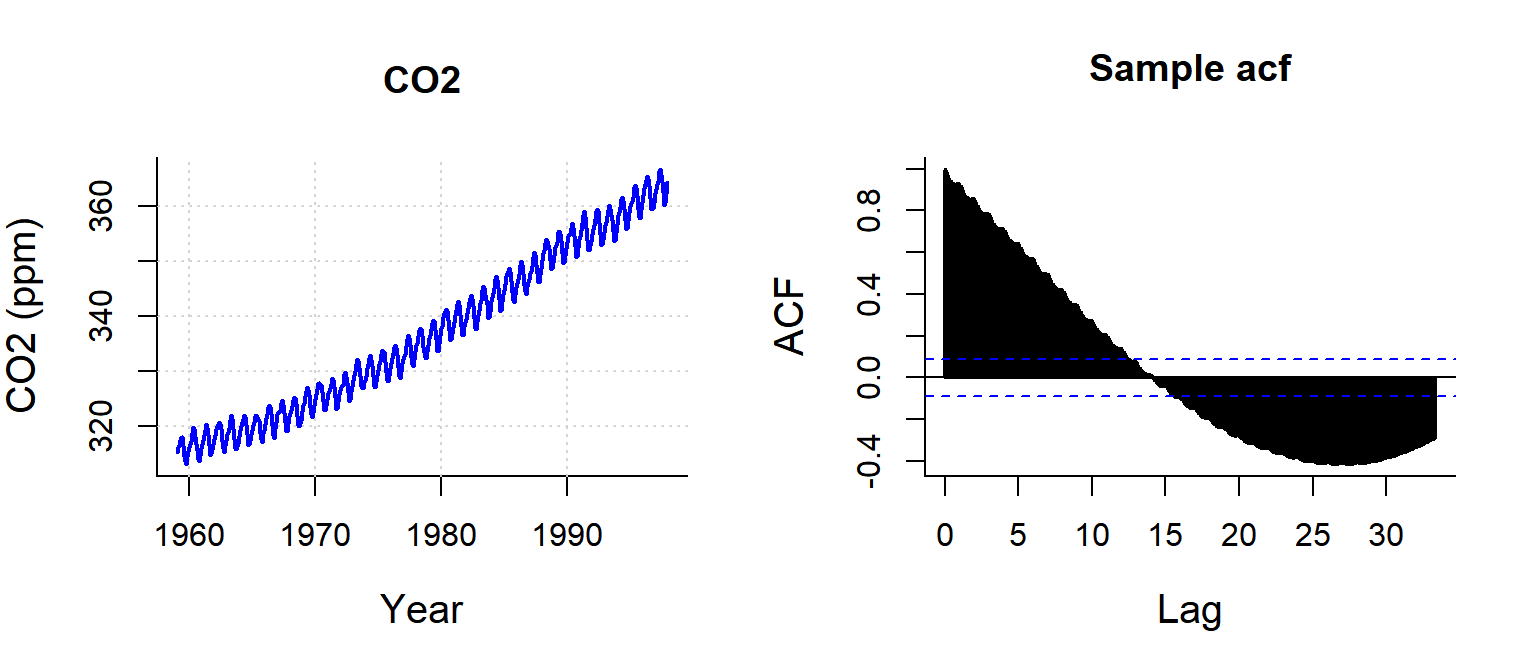
Not useful for time-series with very strong trends!
The autoregression model
First order autoregressive model: AR(1): \[ X_t = \phi_1 \,X_{t-1} + Z_t\] where \(Z_t \sim {\cal N}(0, \sigma^2)\) is White Noise (time series jargon for i.i.d.).
Second order autoregressive: AR(2): \[ X_t = \phi_1 \,X_{t-1} + \phi_2 \, X_{t-2} + Z_t\]
\(p\)-th order autoregressive model: AR(p): \[ X_t = \phi_1 \,X_{t-1} + \phi_2 \, X_{t-2} + ... + \phi_p Z_{t-p} + Z_t \]
Note: these models assume \(\text{E}[X] = 0\). Relaxing this gives (for AR(1)): \[ {X_t = \phi_1 \,(X_{t-1}-\mu) + Z_t + \mu} \]
Pause: to compute \(\text{E}[X]\), \(\text{var}[X]\) and \(\rho(h)\) for an \(X \sim AR(1)\) on the board.
AR(1): Theoretical predictions
\[ \rho(h) = \phi_1^h \]
data(LakeHuron)
acf(LakeHuron)
curve(acf(LakeHuron)$acf[2]^x, add=TRUE, col=3, lwd=2)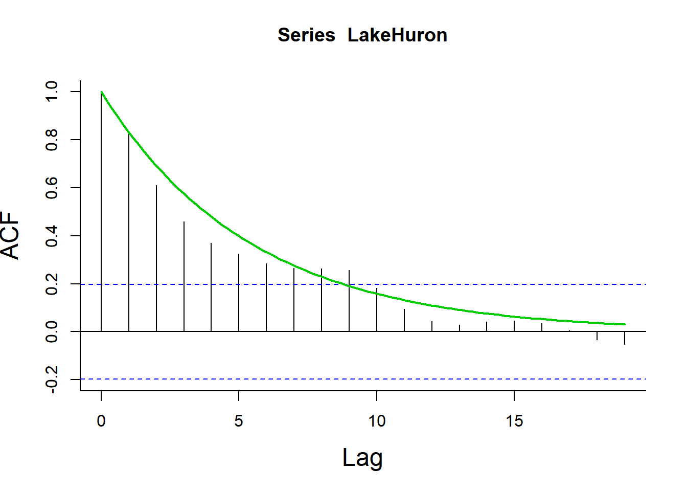
If the sample acf looks exponential - probably an AR(1) model.
Fitting Lake Huron AR(1)
Fit: \({X_t = \phi_1 (\,X_{t-1} - \mu) + Z_t + \mu}\)\
LakeHuron.lm <- lm(LakeHuron[-1] ~ LakeHuron[-length(LakeHuron)])
plot(LakeHuron[-length(LakeHuron)],LakeHuron[-1])
abline(LakeHuron.lm, col=3, lwd=2)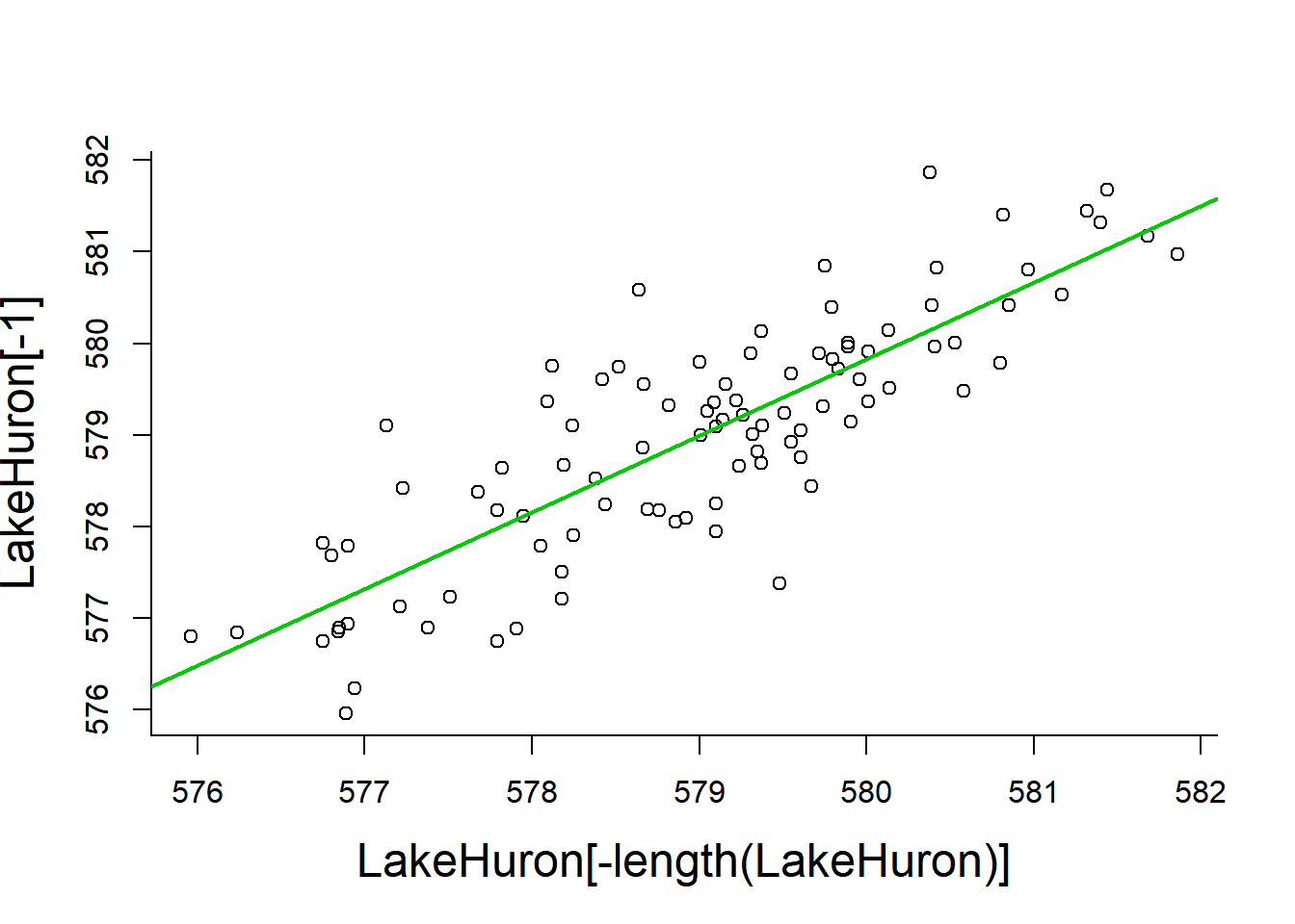
Note: \(R^2 = 0.70\), i.e. about 70% percent of the variation observed in water levels is explained by previous years.
Diagnostic plots
plot(LakeHuron.lm, 1:2)
acf(residuals(LakeHuron.lm))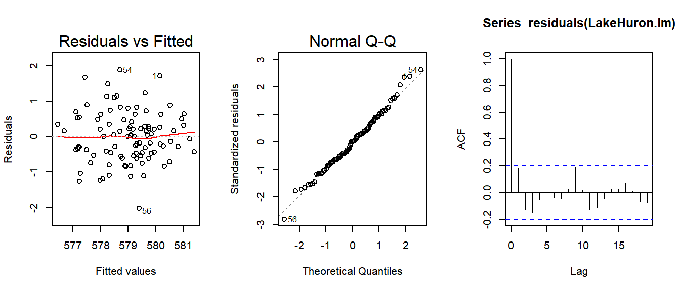
Check regression assumptions: Homoscedastic, Normal, Independent - note use of acf function to test assumption of independence!
But what about the trend?
Decomposition with trend: \[ {Y_t = m_t + X_t} \]
where:
- {\(m_t\) } is the slowly varying trend component
- {\(X_t\) } is a random component
- {\(X_t\)} can have serial autocorrelation
- \(\text{E}[X_t] = 0\)
- \(X_t\) must be stationary.
Definition of Stationary
- \(X_t\) is a Stationary process if \(\text{E}[X_t]\) is independent of \(t\)
- \(X_t\) is what is left over after the time-dependent part is removed
Estimating a trend and correlation to Lake Huron
\[Y_{T} = \beta_0 + \beta_1 T + X_{T}\] \[ X_{T} = \phi_1 X_{T-1} + Z_T \]
plot(LakeHuron, ylab="Level (ft above sea level)", xlab="Year", main="Lake Huron Water Level", col=3, lwd=2)
grid()
lines(LakeHuron, col=3, lwd=1.5)
LH.trend <- lm(LakeHuron~time(LakeHuron))
abline(LH.trend, lwd=2, col="darkred")

acf(residuals(LH.trend), main = "ACF of trend", lag.max=20)
X <- residuals(LH.trend)
X.lm <- lm(X[-1]~X[-length(X)])

summary(X.lm)
##
## Call:
## lm(formula = X[-1] ~ X[-length(X)])
##
## Residuals:
## Min 1Q Median 3Q Max
## -1.95881 -0.49932 0.00171 0.41780 1.89561
##
## Coefficients:
## Estimate Std. Error t value Pr(>|t|)
## (Intercept) 0.01529 0.07272 0.21 0.834
## X[-length(X)] 0.79112 0.06590 12.00 <2e-16 ***
## ---
## Signif. codes: 0 '***' 0.001 '**' 0.01 '*' 0.05 '.' 0.1 ' ' 1
##
## Residual standard error: 0.7161 on 95 degrees of freedom
## Multiple R-squared: 0.6027, Adjusted R-squared: 0.5985
## F-statistic: 144.1 on 1 and 95 DF, p-value: < 2.2e-16acf(residuals(X.lm), main="ACF of residuals of X", lag.max=20)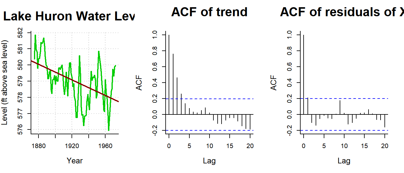
Results:
- \(\widehat{\beta_0} = 625\) ft
- \(\widehat{\beta_1} = -0.024\) ft/year
- \(\widehat{\phi_1} = 0.79\)
- \(\widehat\sigma^2 = 0.513\) ft\(^2\)
Estimating a trend and correlation to Lake Huron
Version 1: Two-step
LH.trend <- lm(LakeHuron ~ time(LakeHuron))
X <- residuals(LH.trend)
X.lm <- lm(X[-1]~X[-length(X)])
summary(X.lm)$coef
## Estimate Std. Error t value Pr(>|t|)
## (Intercept) 0.01528513 0.07272035 0.2101905 8.339691e-01
## X[-length(X)] 0.79111798 0.06590223 12.0044198 9.501693e-21Note the simple linear regression gives a HIGHLY significant result for time.
Version 2: One step
with generalized least squares (gls):
require(nlme)
LH.gls <- gls(LakeHuron ~ time(LakeHuron),
              correlation = corAR1(form=~1))
summary(LH.gls)$tTable
## Value Std.Error t-value p-value
## (Intercept) 616.48869320 24.36263217 25.304683 2.944221e-44
## time(LakeHuron) -0.01943459 0.01266414 -1.534616 1.281674e-01- Correlation coefficient: \(\phi = 0.8247\)
- Regression slope: \(\beta_1 = -0.0194\) - (p-value: 0.13)
WHAT HAPPENED!? The TIME effect is not significant in this model! Does this mean that there is no trend in Lake Huron levels?
Generalized least squares
What DOES ``generalized least squares’’ mean?
Some theoretical background:
Linear regession (“ordinary least squares”):
\[y = {\bf X \beta} + \epsilon\] \(y\) is \(n \times 1\) response, \({\bf X}\) is \(n \times p\) model matrix; \(\beta\) is \(p \times 1\) vector of parameters, \(\epsilon\) is \(n\times 1\) vector of errors. Assuming \(\epsilon \sim {\cal N}(0, \sigma^2 {\bf I}_n)\) (where \({\bf I}_n\) is \(n\times n\) identity matrix) gives {} estimator of \(\beta\): \[\hat{\beta} = ({\bf X}'{\bf X})^{-1}{\bf X}'y \] \[V(\hat{\beta}) = \sigma^2 ({\bf X}'{\bf X})^{-1}\]
Solving this is the equivalent of finding the \(\beta\) that minimizes the Residual Sum of Squares: \[ RSS(\beta) = \sum_{i=1}^n (y_i - {\bf X}_i \beta)^2\]
Assume more generally that \(\epsilon \sim {\cal N}(0, \Sigma)\) has nonzero off-diagonal entries corresponding to correlated errors. If \(\Sigma\) is known, the log-likelihood for the model is maximized with:
\[\hat{\beta}_{gls} = ({\bf X}\Sigma^{-1}{\bf X})^{-1} {\bf X} \Sigma^{-1}{\bf y}\]
For example, when \(\Sigma\) is a diagonal matrix of unequal error variances (heteroskedasticity), then \(\hat{\beta}\) is the weighted-least-squares (WLS) estimator.
In a real application, of course, \(\Sigma\) is not known, and must be estimated along with the regression coefficients \(\beta\) … But there are way too many elements in \(\Sigma\) - (this many: $ n (n+1) / 2 $).
A large part of dealing with dependent data is identifying a tractable, relatively simple form for that residual variance-covariance matrix, and then solving for the coefficients.
This is: generalized least squares} (GLS)
Visualizing variance-covariance matrices:
Empirical \(\Sigma\) matrix and theoretical \(\Sigma\) matrix for residuals\
# Empirical Sigma
res <- lm(LakeHuron~time(LakeHuron))$res
n <- length(res); V <- matrix(NA, nrow=n, ncol=n)
for(i in 1:n) V[n-i+1,(i:n - i)+1] <- res[i:n]
ind <- upper.tri(V); V[ind] <- t(V)[ind]

# Fitted Sigma
sigma.hat <-  LH.gls$sigma
phi.hat <- 0.8
require(lattice)
V.hat <- outer(1:n, 1:n, function(x,y) phi.hat^abs(x-y))
require(fields); image.plot(var(V)); image.plot(sigma.hat*V.hat)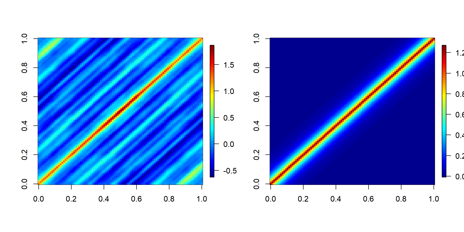
How to determine the order of an AR(p) model?
The base ar() function, which uses AIC.
Raw lake Huron data:
ar(LakeHuron)##
## Call:
## ar(x = LakeHuron)
##
## Coefficients:
## 1 2
## 1.0538 -0.2668
##
## Order selected 2 sigma^2 estimated as 0.5075Residuals of time regression:
LH.lm <- lm(LakeHuron~time(LakeHuron))
ar(LH.lm$res)
##
## Call:
## ar(x = LH.lm$res)
##
## Coefficients:
## 1 2
## 0.9714 -0.2754
##
## Order selected 2 sigma^2 estimated as 0.501Or you can always regress by hand against BOTH orders:
n <- length(LakeHuron)
summary(lm(LH.lm$res[3:n] ~
           LH.lm$res[2:(n-1)] +
           LH.lm$res[1:(n-2)]))
##
## Call:
## lm(formula = LH.lm$res[3:n] ~ LH.lm$res[2:(n - 1)] + LH.lm$res[1:(n -
## 2)])
##
## Residuals:
## Min 1Q Median 3Q Max
## -1.58428 -0.45246 -0.01622 0.40297 1.73202
##
## Coefficients:
## Estimate Std. Error t value Pr(>|t|)
## (Intercept) -0.007852 0.069121 -0.114 0.90980
## LH.lm$res[2:(n - 1)] 1.002137 0.097215 10.308 < 2e-16 ***
## LH.lm$res[1:(n - 2)] -0.283798 0.099004 -2.867 0.00513 **
## ---
## Signif. codes: 0 '***' 0.001 '**' 0.01 '*' 0.05 '.' 0.1 ' ' 1
##
## Residual standard error: 0.6766 on 93 degrees of freedom
## Multiple R-squared: 0.6441, Adjusted R-squared: 0.6365
## F-statistic: 84.17 on 2 and 93 DF, p-value: < 2.2e-16In either case, strong evidence of a NEGATIVE second-order correlation. (note \(\phi_1 > 1\)!)
Fitting an AR(2) model with gls
\[Y_i = \beta_0 + \beta_1 T_i + \epsilon_i\] \[\epsilon_i = AR(2)\]
require(nlme)
LH.gls2 <- gls(LakeHuron ~ time(LakeHuron), correlation = corARMA(p=2))
summary(LH.gls2)
## Generalized least squares fit by REML
## Model: LakeHuron ~ time(LakeHuron)
## Data: NULL
## AIC BIC logLik
## 221.028 233.8497 -105.514
##
## Correlation Structure: ARMA(2,0)
## Formula: ~1
## Parameter estimate(s):
## Phi1 Phi2
## 1.0203418 -0.2741249
##
## Coefficients:
## Value Std.Error t-value p-value
## (Intercept) 619.6442 17.491090 35.42628 0.0000
## time(LakeHuron) -0.0211 0.009092 -2.32216 0.0223
##
## Correlation:
## (Intr)
## time(LakeHuron) -1
##
## Standardized residuals:
## Min Q1 Med Q3 Max
## -2.16624672 -0.57959971 0.01070681 0.61705337 2.03975934
##
## Residual standard error: 1.18641
## Degrees of freedom: 98 total; 96 residualCorrelation coefficients: - \(\phi_1 = 1.02\)\ - \(\phi_2 = -0.27\)\
Regression slope: \ - \(\beta_1 = -0.021\) - p-value: 0.02\
So …. by taking the second order autocorrelation into account the temporal regression IS significant!?
Comparing models …
LH.gls0.1 <- gls(LakeHuron ~ 1, correlation = corAR1(form=~1), method="ML")
LH.gls0.2 <- gls(LakeHuron ~ 1, correlation = corARMA(p=2), method="ML")
LH.gls1.1 <- gls(LakeHuron ~ time(LakeHuron), correlation = corAR1(form=~1), method="ML")
LH.gls1.2 <- gls(LakeHuron ~ time(LakeHuron), correlation = corARMA(p=2), method="ML")

anova(LH.gls0.1, LH.gls0.2, LH.gls1.1, LH.gls1.2)
## Model df AIC BIC logLik Test L.Ratio p-value
## LH.gls0.1 1 3 219.1960 226.9509 -106.5980
## LH.gls0.2 2 4 215.2664 225.6063 -103.6332 1 vs 2 5.929504 0.0149
## LH.gls1.1 3 4 218.4502 228.7900 -105.2251
## LH.gls1.2 4 5 212.3965 225.3214 -101.1983 3 vs 4 8.053612 0.0045THe lowest AIC - by a decent-ish margin - is the second order model with lag.
Note the non-default method = "ML" means that we are Maximizing the Likelihood (as opposed to the default, faster REML - restricted likelihood - which fits parameters but is harder to compare models with)
Newest conclusions:
- The water level in Lake Huron IS dropping, and there is a high first order and significant negative second-order auto-correlation to the water level.
- Even for very simple time-series and questions about simple linear trends … it is easy to make false inference (both see patterns that are not there, or fail to detect patterns that are there) if you don’t take auto-correlations into account!
An important twist: Moving average models
First-order moving average model: MA(1) \[ Z_t = Z_t + \psi Z_{t-1} \] i.e. the “random shock” (aka “innovation”) depends on the previous “random shock”.
\(q\)-th order moving average model: MA(\(q\)) \[\epsilon_t = \psi_1 \,Z_{t-1} + \psi_2 \, Z_{t-2} + ... + \psi_q Z_{t-q} + Z_t\]
Assessed via the {} \[\phi(k) =\mathop{\text{Corr}}(X_t-{\cal P}(X_t\mid X_{t+1},\ldots,X_{t+k-1}) \qquad X_{t+k}-{\cal P}(X_{t+k}\mid X_{t+1},\ldots,X_{t+k-1}))\]
where: \({\cal P}(Y\mid X)\) is the best linear projection of \(Y\) on \(X\), i.e.~we’ve regressed away all of the lags and are left only with the cross-correlation of the residuals.
PACF(h) of an AR(1) is 0 at \(h>0\)
phi <- 0.8; nu <- rnorm(100)
esp.AR <- c(rnorm(1),rep(NA,100))
for(i in 1:100) esp.AR[i+1] <- phi*esp.AR[i] + nu[i]
pacf(esp.AR, main="pacf")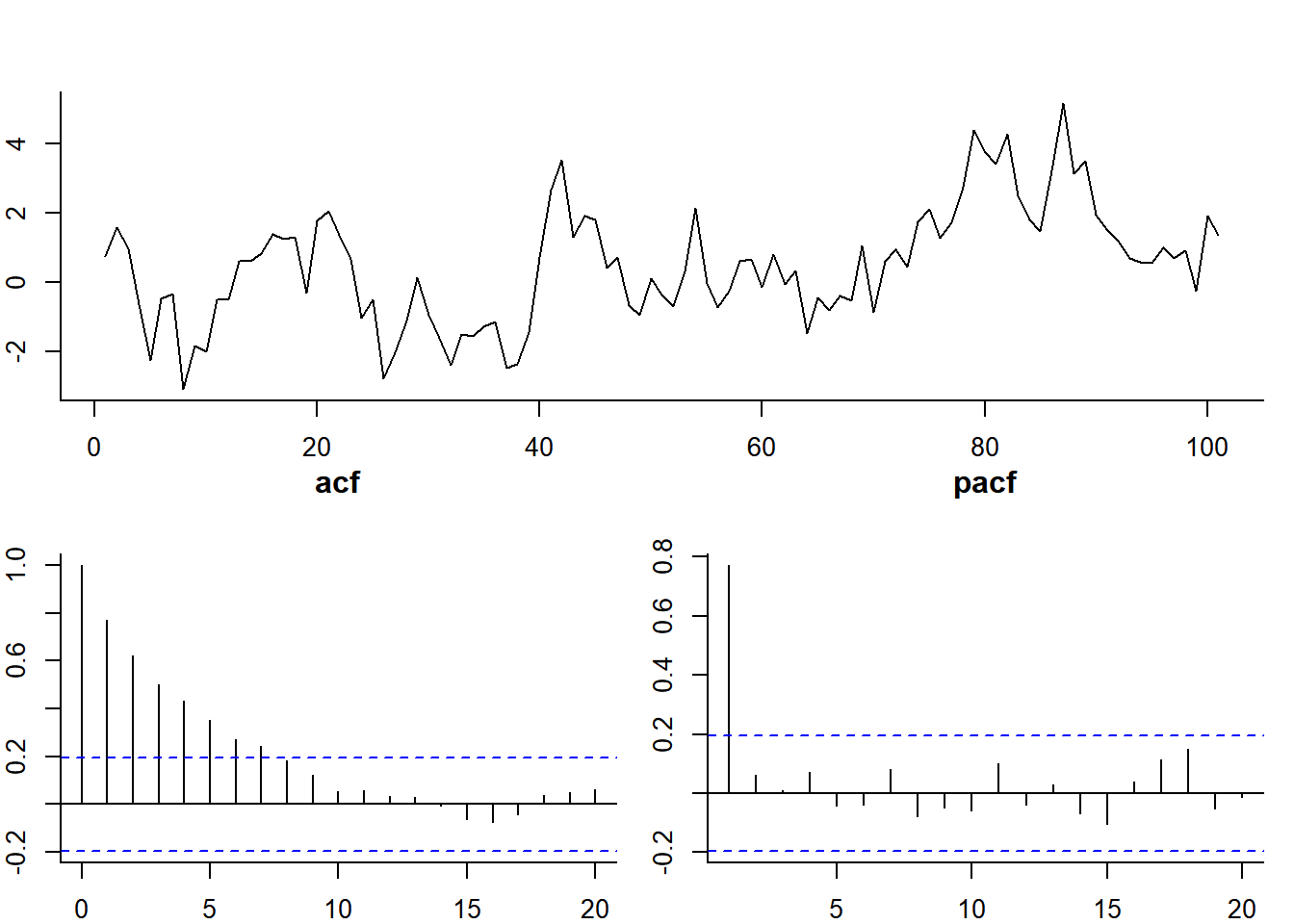
ACF(h) of an MA(1) is 0 at \(h>1\)
psi <- 0.8;  nu <- rnorm(101)
esp.MA <- c(rnorm(1),rep(NA,100))
for(i in 2:101) esp.MA[i] <- nu[i] + psi*nu[i-1]
pacf(esp.MA, main="pacf")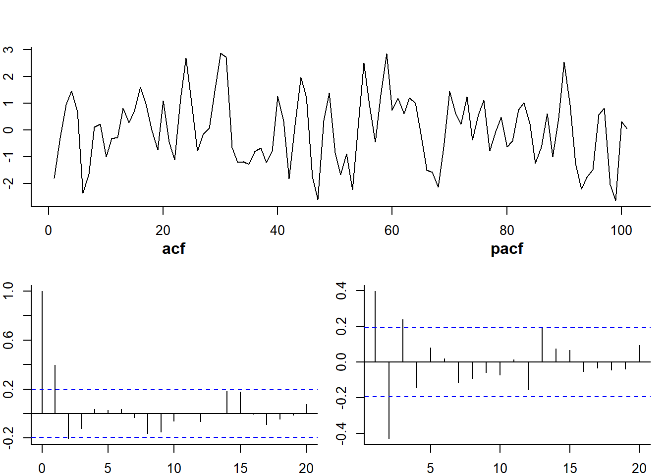
ARMA(p,q) model
Y <- arima.sim(model = list(ar = c(0.9, -.5), ma = c(-2,-4)), 1000)
A lot of the traditional wizardry of time-series analysis is looking at acf’s and pacf’s and deducing the ARMA model.
Selecting ARMA(p,q)
We can just ask AIC to help us out.
get.aic.table <- function(Y){
aic.table <- AIC(
  arima(Y, c(1,0,0)), arima(Y, c(0,0,1)), arima(Y, c(1,0,1)), arima(Y, c(2,0,0)), arima(Y, c(0,0,2)),
  arima(Y, c(1,0,2)),  arima(Y, c(2,0,1)), arima(Y, c(2,0,2)), arima(Y, c(3,0,2)), arima(Y, c(3,0,3)))
aic.table[order(aic.table$AIC),]
}
Y <- arima.sim(model =
list(ar = c(0.9, -.5),
ma = c(-2,-4)), 1000)
get.aic.table(Y)## df AIC
## arima(Y, c(2, 0, 2)) 6 5598.706
## arima(Y, c(3, 0, 2)) 7 5599.602
## arima(Y, c(3, 0, 3)) 8 5601.606
## arima(Y, c(2, 0, 1)) 5 5612.976
## arima(Y, c(1, 0, 2)) 5 5671.705
## arima(Y, c(0, 0, 2)) 4 5672.147
## arima(Y, c(1, 0, 1)) 4 5747.617
## arima(Y, c(2, 0, 0)) 4 5807.243
## arima(Y, c(0, 0, 1)) 3 5916.302
## arima(Y, c(1, 0, 0)) 3 6361.015get.aic.table(LakeHuron)## df AIC
## arima(Y, c(1, 0, 1)) 4 214.4905
## arima(Y, c(2, 0, 0)) 4 215.2664
## arima(Y, c(1, 0, 2)) 5 216.4645
## arima(Y, c(2, 0, 1)) 5 216.4764
## arima(Y, c(2, 0, 2)) 6 218.4106
## arima(Y, c(1, 0, 0)) 3 219.1959
## arima(Y, c(3, 0, 2)) 7 219.6967
## arima(Y, c(3, 0, 3)) 8 221.1937
## arima(Y, c(0, 0, 2)) 4 230.9306
## arima(Y, c(0, 0, 1)) 3 255.2950get.aic.table(LH.lm$res)## df AIC
## arima(Y, c(2, 0, 0)) 4 210.5032
## arima(Y, c(1, 0, 1)) 4 210.5176
## arima(Y, c(1, 0, 2)) 5 212.1225
## arima(Y, c(2, 0, 1)) 5 212.1784
## arima(Y, c(2, 0, 2)) 6 214.1224
## arima(Y, c(3, 0, 2)) 7 215.2280
## arima(Y, c(1, 0, 0)) 3 216.5835
## arima(Y, c(3, 0, 3)) 8 216.6927
## arima(Y, c(0, 0, 2)) 4 217.8177
## arima(Y, c(0, 0, 1)) 3 235.2032Note that any MA effects get (mostly) explained away by accounting for the time trend.
Forecasting
require(forecast)
(LH.forecast <- forecast(Arima(LH.lm$res, order = c(2,0,0), include.mean=FALSE)))
## Point Forecast Lo 80 Hi 80 Lo 95 Hi 95
## 99 1.545023949 0.6695495 2.420498 0.2061013 2.883947
## 100 0.929893256 -0.3113219 2.171108 -0.9683815 2.828168
## 101 0.482673894 -0.9084677 1.873816 -1.6448936 2.610241
## 102 0.213122974 -1.2274235 1.653669 -1.9900028 2.416249
## 103 0.073021289 -1.3802861 1.526329 -2.1496206 2.295663
## 104 0.011054189 -1.4446636 1.466772 -2.2152740 2.237382
## 105 -0.010247304 -1.4662334 1.445739 -2.2369859 2.216491
## 106 -0.013531751 -1.4695223 1.442459 -2.2402771 2.213214
## 107 -0.010602506 -1.4666002 1.445395 -2.2373588 2.216154
## 108 -0.006697958 -1.4627065 1.449311 -2.2334709 2.220075plot(LH.forecast)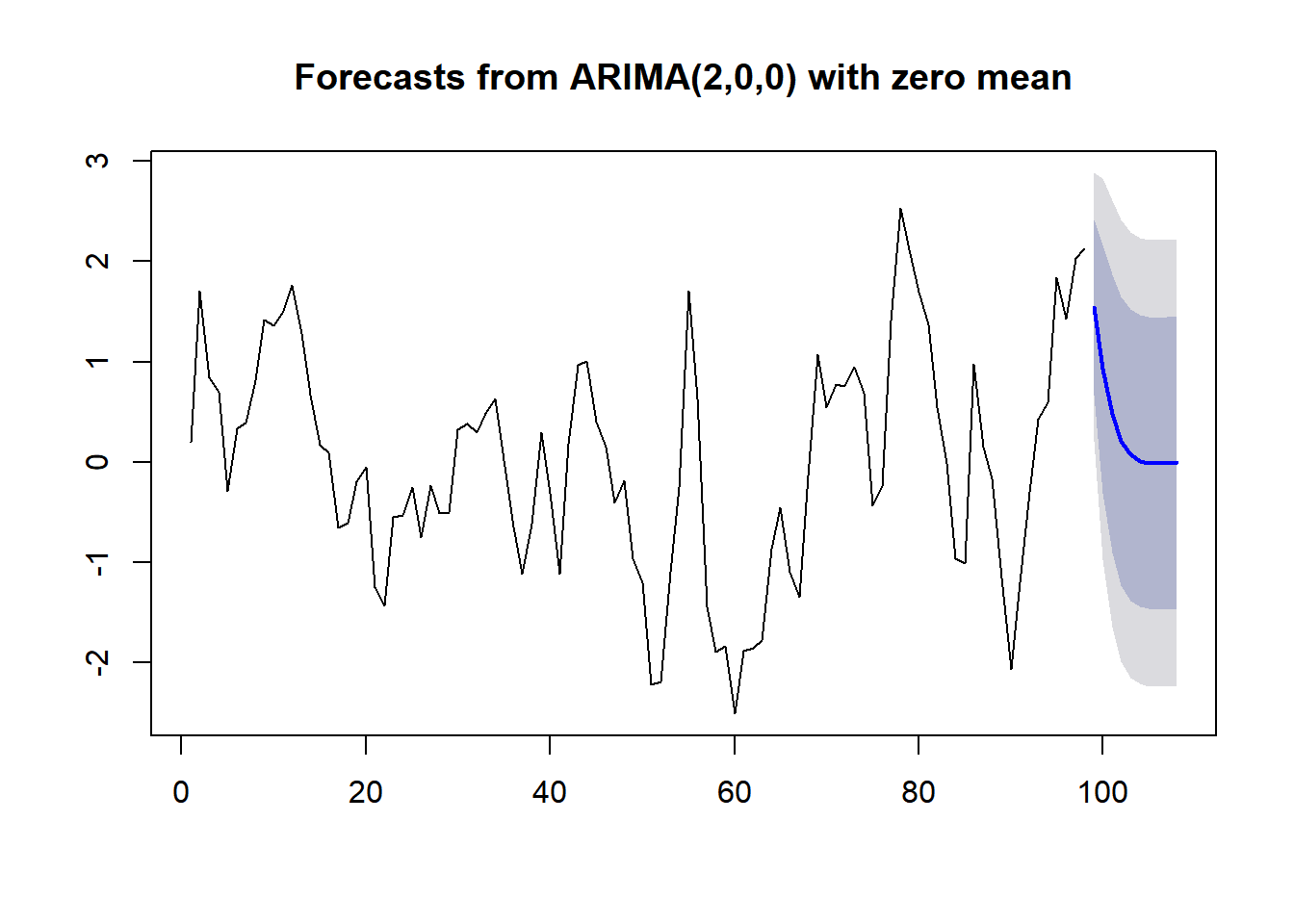
Forecasting with trend: (with apologies for ugly code)
plot(LakeHuron, xlim=c(1870,2012), ylim=c(570,585))
T.new <- 1972:2000
LH.forecast <- forecast(Arima(LH.lm$res, order = c(2,0,0), include.mean=FALSE), h=length(T.new))
T <- as.numeric(time(LakeHuron))

LH.lm <- lm(as.numeric(LakeHuron)~T)
LH.predict <- predict(LH.lm, newdata = list(T = T.new))

lines(T.new, LH.predict + LH.forecast$mean, col=2)
polygon(c(T.new,  T.new[length(T.new):1]), c(LH.predict + LH.forecast$lower[,1], (LH.predict + LH.forecast$upper[,1])[length(T.new):1]), col=rgb(0,0,1,.2), bor=NA)
polygon(c(T.new,  T.new[length(T.new):1]), c(LH.predict + LH.forecast$lower[,2], (LH.predict + LH.forecast$upper[,2])[length(T.new):1]), col=rgb(0,0,1,.2), bor=NA)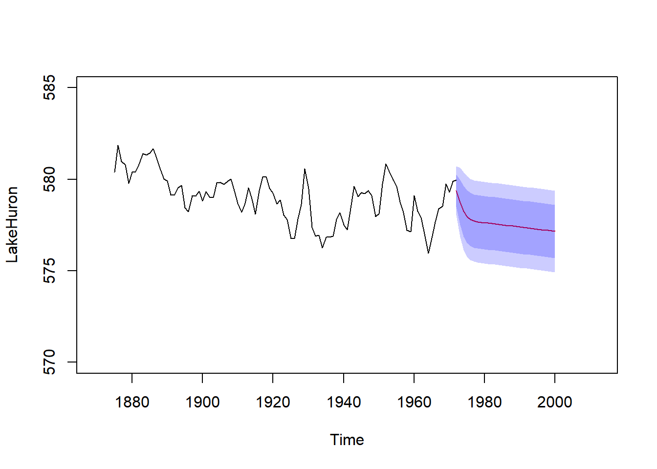
Out of curiousity, I downloaded the Lake Huron water levels up to 2012 from :
LH <- read.csv("../_data/miHuron1918Ann.csv")
par(bty="l", cex.lab=1.25, las=1)
plot(LakeHuron, xlim=c(1870,2017), ylim=c(572,585), ylab="Lake Huron water level (feet)")
T.new <- 1972:2017
LH.forecast <- forecast(Arima(LH.lm$res, order = c(2,0,0), include.mean=FALSE), h=length(T.new))
T <- as.numeric(time(LakeHuron))

LH.lm <- lm(as.numeric(LakeHuron)~T)
LH.predict <- predict(LH.lm, newdata = list(T = T.new))

lines(T.new, LH.predict + LH.forecast$mean, col="darkblue")
polygon(c(T.new,  T.new[length(T.new):1]), c(LH.predict + LH.forecast$lower[,1], (LH.predict + LH.forecast$upper[,1])[length(T.new):1]), col=rgb(0,0,1,.2), bor=NA)
polygon(c(T.new,  T.new[length(T.new):1]), c(LH.predict + LH.forecast$lower[,2], (LH.predict + LH.forecast$upper[,2])[length(T.new):1]), col=rgb(0,0,1,.2), bor=NA)

lines(LH$year, LH$AnnAvg*3.28084, type="l", col=2, lwd=2)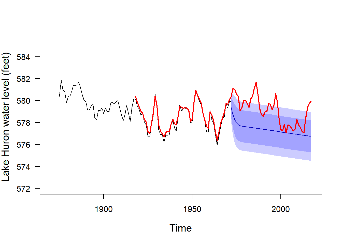
Conclusion? This is a time series with a weak trend and lots of variability - forecasting won’t give you much, except perhaps in the very short term.
But the question is important: http://research.noaa.gov/News/NewsArchive/LatestNews/TabId/684/ArtMID/1768/ArticleID/10466/NOAA-Seeks-Answers-to-Great-Lakes-Water-Level-Changes--.aspx

Classical Decomposition, with trend and seasonality
\[ {Y_t = m_t + s_t + X_t} \]
where:
- \(m_t\) is the component
- \(s_t\) is the component
- \(s_{t+d} = s_t\), where \(d\) is the
- Usually, we know the period \(d\) (and do not need to estimate it)
- \(X_t\) is a random component, that is (hopefully) stationary
- Usually, we know the period \(d\) (and do not need to estimate it)
CO2 data from Mauna Loa
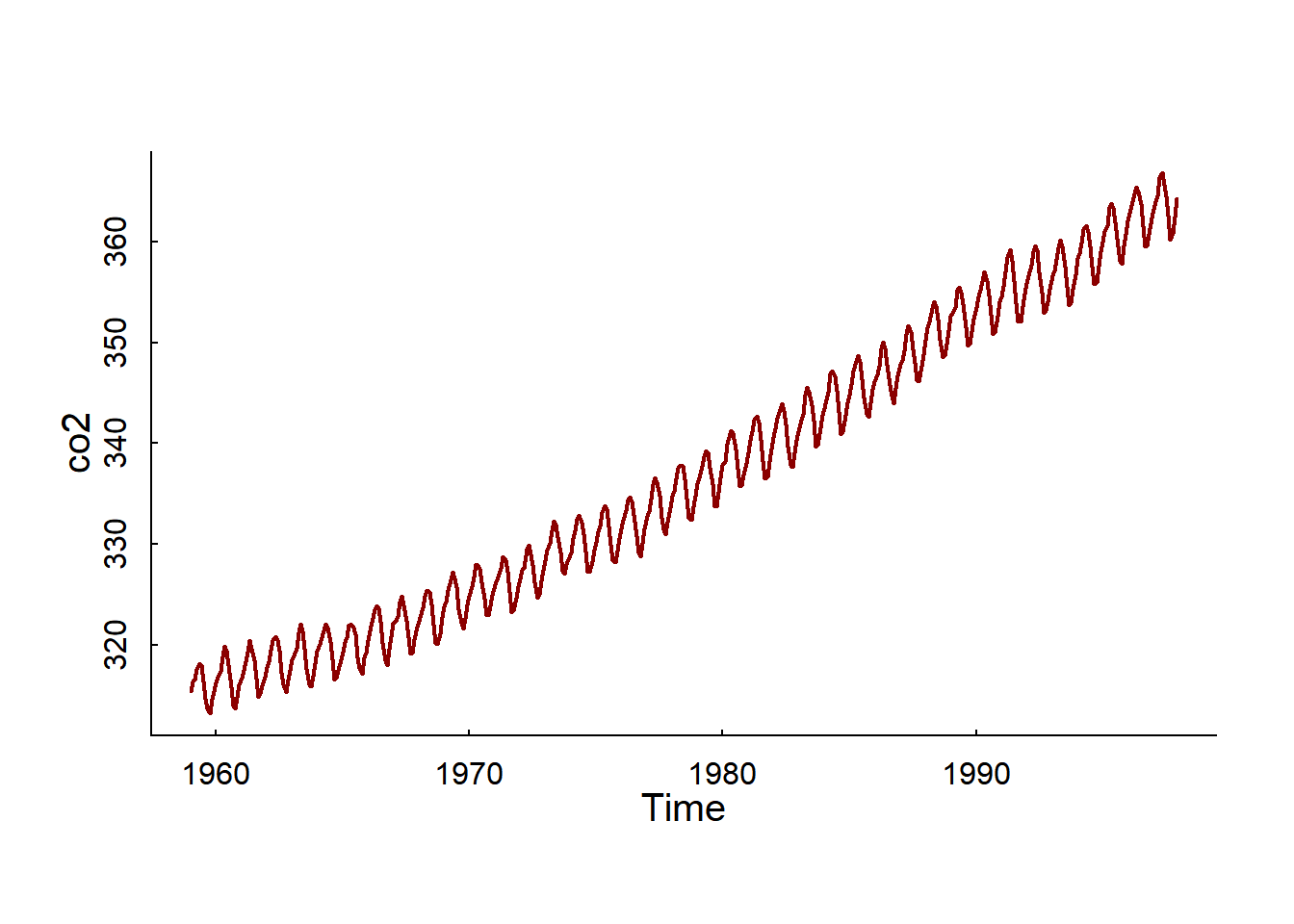
Linear detrending
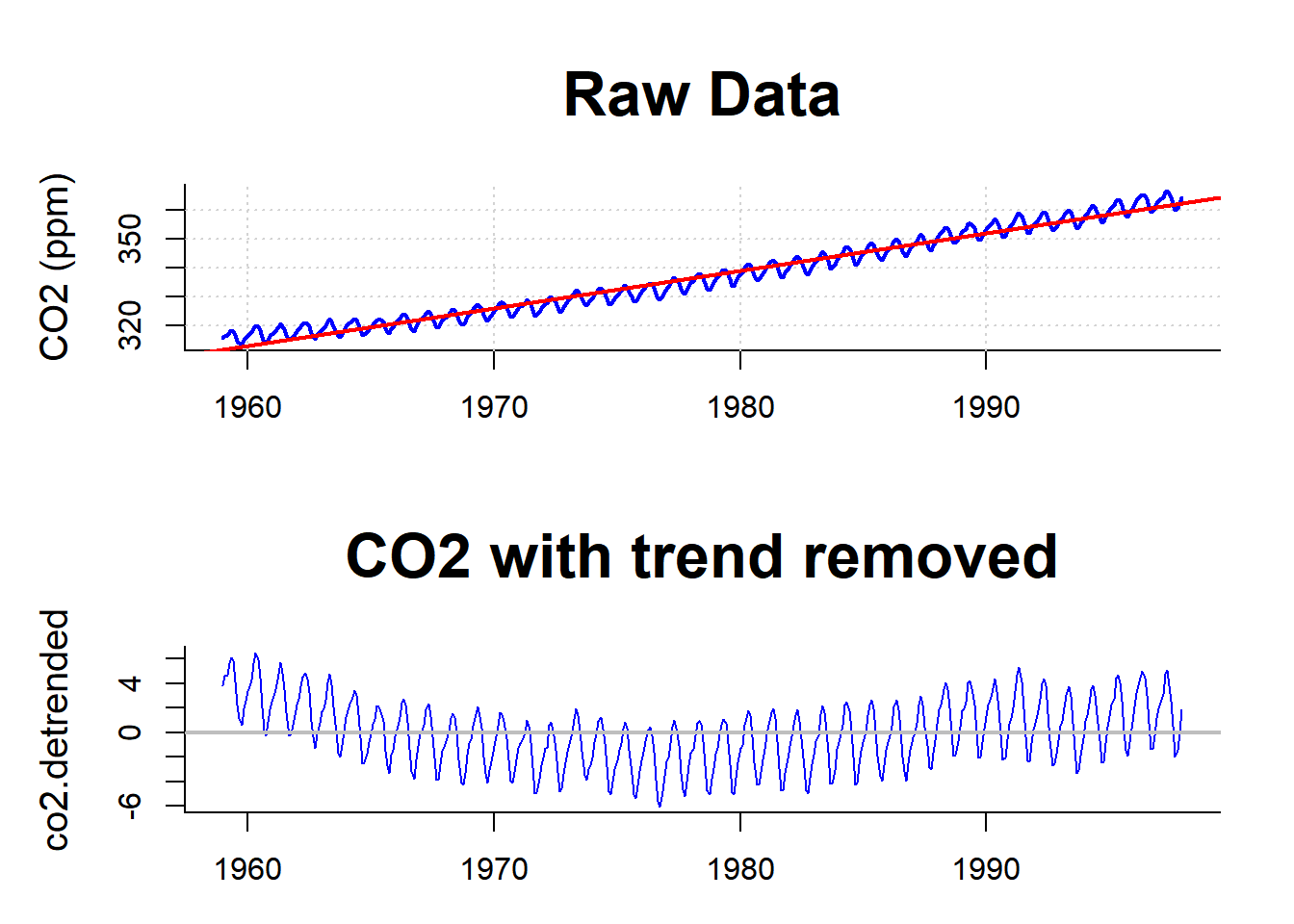
Not very satisfactory
“Classical” decomposition of CO2 data
\[Y_t = m_t + s_t + X_t}\]
Key bits of code (try this at home!):
# time series objects have "time" attributes
  t <- as.vector(time(co2))
  co2.lm <- lm(co2 ~ poly(t, 3))
  Y.trend <-  predict(co2.lm)
# tapply to average away at "cycle" of periodic  data
  co2.detrended <- co2 - Y.trend
  st <- tapply(co2.detrended, cycle(co2), mean)
  Y.seasonal <- st[cycle(co2)]
# random component
  Y.random <- co2.detrended - Y.seasonal
- \(m_t\): fit a cubic polynomial
- obtain detrended series: \(V_t = Y_t - m_t\).
- Seasonal component: \(s_{t+i} = {1\over 12} \sum\limits_{d=1}^{n/d} V_{t+d+i}\)
- Random componenent: \(X_t = AR(p)\)
One line in R: decompose()
plot(decompose(co2))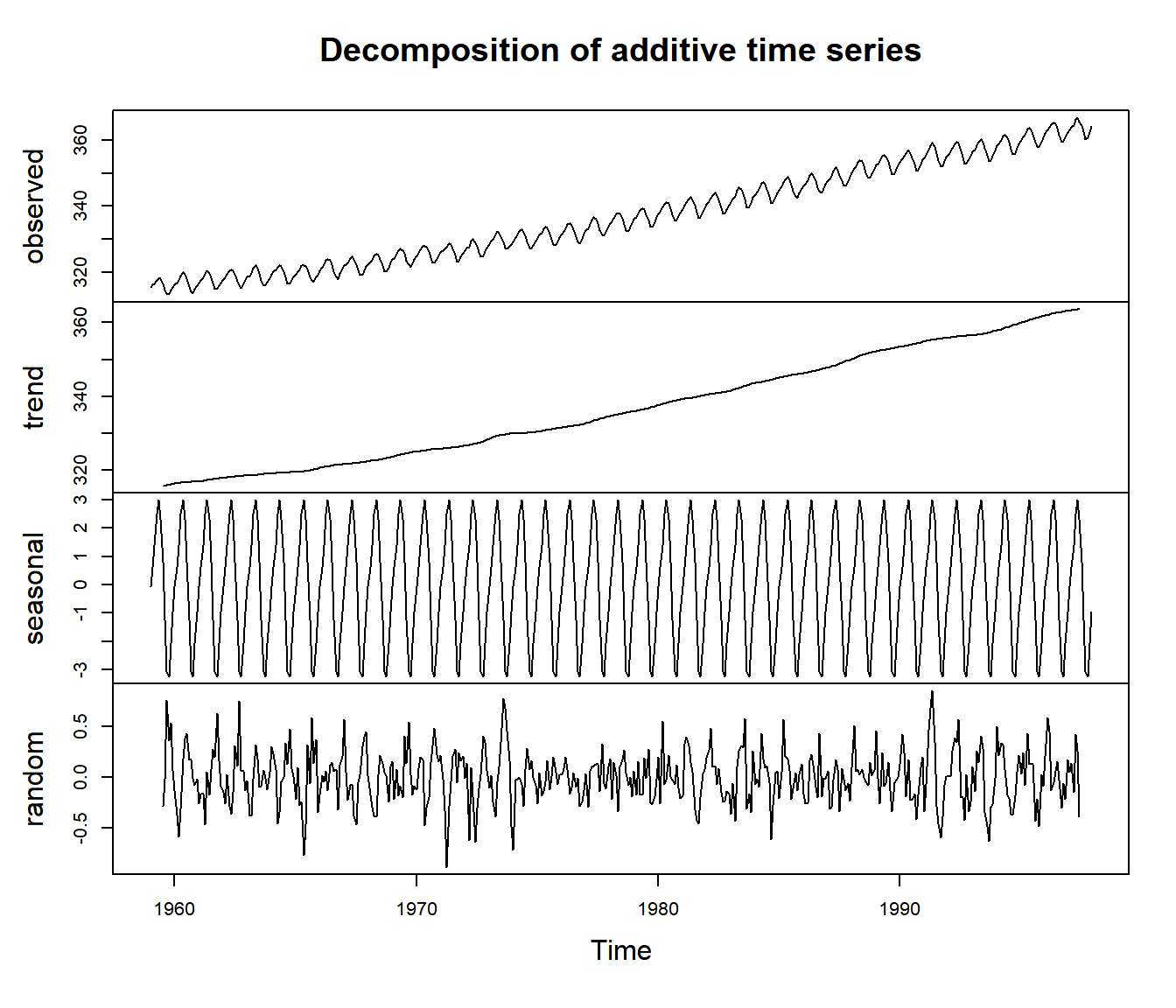
Note: The trend term here is non-parametric, but a moving window filter (size \(d\)): \[ m_t = {1 \over 2} \sum_{i = t-d/2}^{t+d/2} Y_{i} \] This is a good smoothing technique, but not useful for prediction
A caution about polynomial fits:
They look great in the region they are fitting …
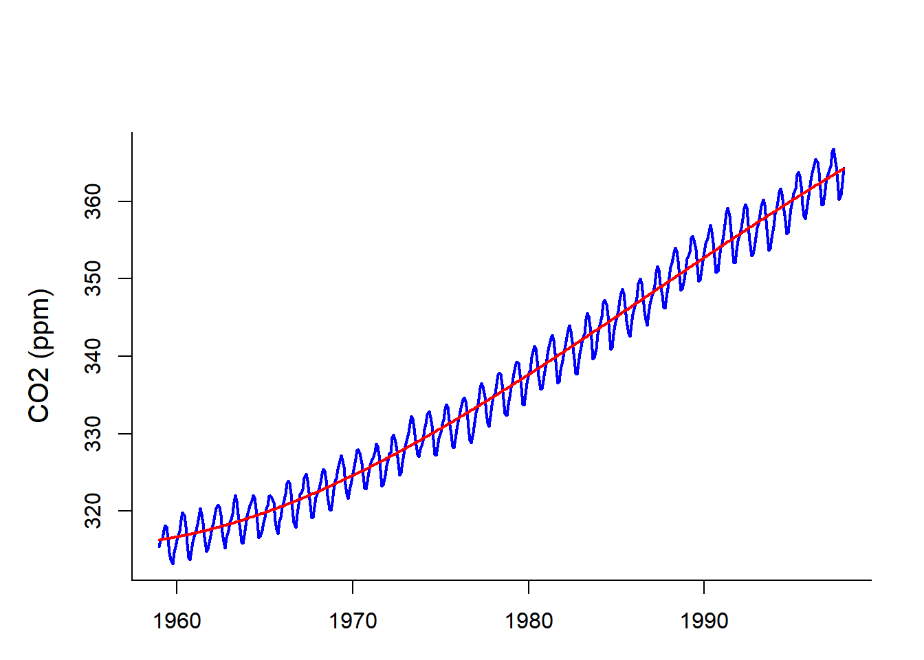
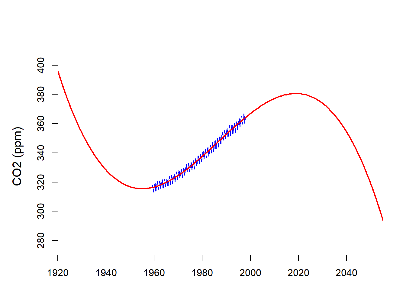
but the better they fit, the less reliable they are far away.
Incidentally:
In 2013, CO2 at Mauna Loa hit 400 ppm for the first time

In 2016, CO2 went over 400 ppm permanently.

How well could we have predicted that from our time-series model?
Population cycles


Cross-correlation functions
Recall autocorrelation:
- Autocorrelation function: \(\rho(h) = {\text{E}[(X_t - \mu_x)(Y_{t+h} - \mu_y)] \over \sigma_x^2}\)
- Sample autocorrelation: {\(\widehat{\gamma}(h) = {1 \over n s_x^2} \sum_{t=1}^{n-|h|} (X_{t+|h|} - \overline{X})(X_t - \overline{X})\)}
Analogously:
- Cross-correlation function: \[ \rho_{xy}(h) = {\text{E}[(X_t - \mu_x)(Y_{t+h} - \mu_y)] \over \sigma_x \sigma_y} \]
- Sample cross-correlation: \[ \widehat{\gamma}(h) = {1 \over n s_x s_y} \sum_{t=1}^{n-|h|} (Y_{t+|h|} - \overline{X})(X_t - \overline{X})\]
Cross-correlation allows identification of relationships BETWEEN time-series over different lags.
Cross-correlation of lynx and hare
In R, simply: ccf(Hare, Lynx)
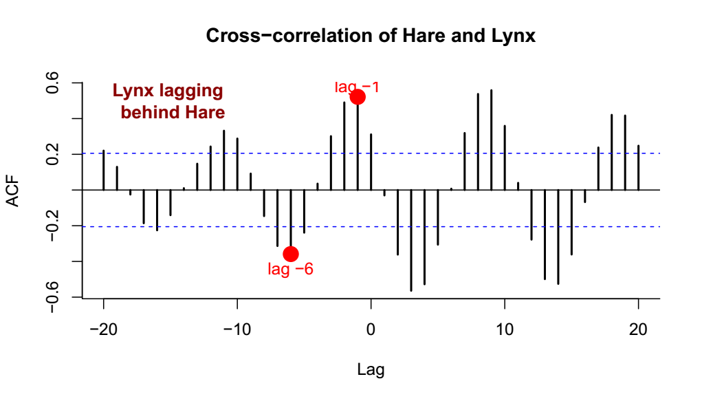

Which of these effects is more important: Less Lynx leads to more Hare? More Hare leads to more Lynx? More Lynx leads to less Hare? Less Hare leads to less Lynx? These are difficult, but not impossible, questions to parse!
Some intermediate conclusions
- If you do not account for correlation in your data, it is easy to make false inferences…
- BUT, there are interesting things to be learned from studying the (terrifying) lack of independence.
- A general strategy is to systematically extract all the patterns or otherwise reduce the data until you have extracted the stationary piece.
- Many basic concepts from regression are useful.
- There are many easy-to-use tools in R (and elsewhere) that, like Virgil, hold your hand as you make your journey through the inferno of dependent data.
- There are many ways to slice a time-series! As with any analysis - you have to be persistent and dig around and be creative.
In final conclusion

Additional Resource
The main R guru for time series is Rob Hyndman, author of the forecast package.
See the CRAN Task View: Time Series Analysis for many many packages related to time series analysis.
An important ones (that I use and that we’ll use in lab) is: zoo.