Maximizing Likelihoods For Mixed Distributions
BIOL709/BSCI339
The Data
Let’s say you have a bi-modal distribution and you want to a mixture model of normals. As a motivating example, see the Old Faithful data:
data(faithful)
head(faithful)
## eruptions waiting
## 1 3.600 79
## 2 1.800 54
## 3 3.333 74
## 4 2.283 62
## 5 4.533 85
## 6 2.883 55waiting <- faithful$waiting
h <- hist(waiting, col="grey", bor = "darkgrey", breaks=20, prob=TRUE,
xlab = "Waiting time between eruptions (min)", main="")
lines(density(waiting), col=2, lwd=2)
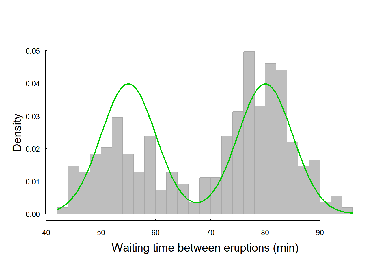
It looks like the distribution here might be a mixture of two normals, i.e. that there are two types of processes that lead to eruption - a short one, and a long one - each with its own mean and variance. We could write that distribution as follows: \[f(w) = \alpha \phi(w, \mu_1, \sigma_1) + (1-\alpha) \phi(w, \mu_2, \sigma_2)\] where \(\phi\) is the normal distribution, and \(\alpha\) is the percentage of times the eruption occurs with the first or second waiting time process.
We can define this distribution function, and try to eyeball its fit - the means are around 55 and 80, the standard deviations are, maybe, 5, the proportions about 50-50:
# the function
mixed.dnorm <- function(x, alpha, mu1, sigma1, mu2, sigma2)
  alpha*dnorm(x, mu1, sigma1) + (1-alpha)*dnorm(x, mu2, sigma2)

hist(waiting, col="grey", bor = "darkgrey", breaks=20, prob=TRUE,
     xlab = "Waiting time between eruptions (min)", main="")

curve(mixed.dnorm(x, 0.5, 55, 5, 80, 5), add=TRUE, col=3, lwd=2)
It is a decent, but not great, guess.
The Likelihood
Lets fit this with a likelihood:
ll.mixed.dnorm <- function(p, X){
  logLs <- log(mixed.dnorm(x = X, alpha = p["alpha"],
                          mu1 = p["mu1"], sigma1 = p["sigma1"],
                          mu2 = p["mu2"], sigma2 = p["sigma2"]))
  return(-sum(logLs))
}
Something to note about this code: in previous examples, I’ve extracted each parameter in the vector of parameters p, e.g.: mu <- p[1]; sigma <- p[2], etc. But in this case, as long as the parameters are named, you don’t need to keep track of the order of your parameters, and the output of optim will make it easier to see what they are.
So, now we fit the data, using our initial parameters as a guess:
p0 <- c(alpha = 0.5, mu1 = 55, mu2 = 80, sigma1 = 5, sigma2 = 5)
(waiting.fit <- optim(p0, ll.mixed.dnorm, X = waiting, hessian=TRUE))$par
## alpha mu1 mu2 sigma1 sigma2
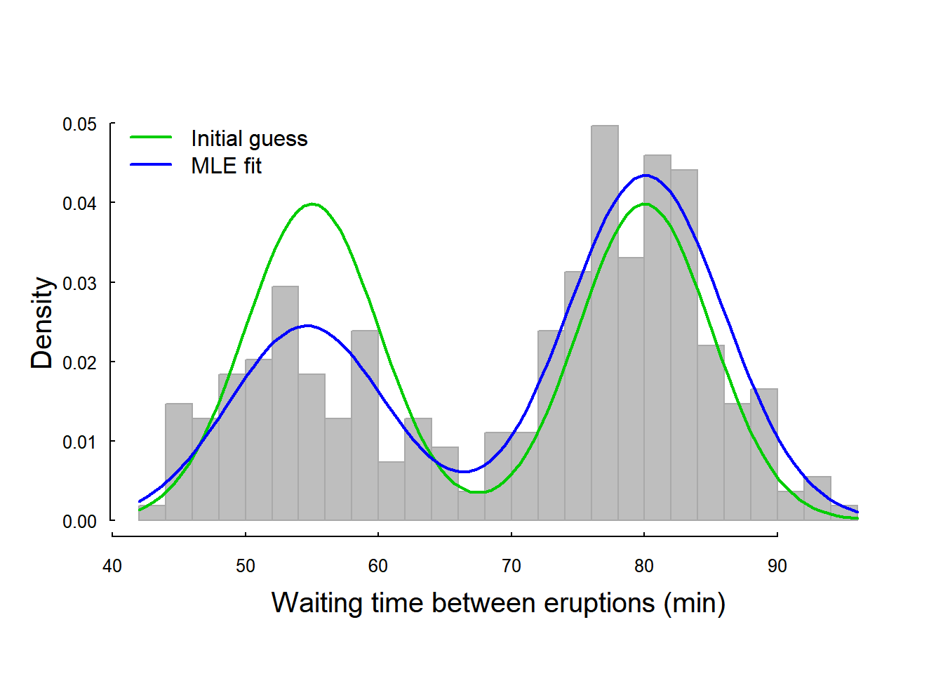
## 0.3607643 54.6148910 80.0922823 5.8704523 5.8685722These look like reasonable estimates: about 36% of time in the first state, the means were pretty close, the variances a bit larger than predicted. We visualize the fit below:
hist(waiting, col="grey", bor = "darkgrey", breaks=20, prob=TRUE,
     xlab = "Waiting time between eruptions (min)", main="")
with(as.list(p0),
      curve(mixed.dnorm(x, alpha, mu1, sigma1, mu2, sigma2), add=TRUE, col=3, lwd=2))
with(as.list(waiting.fit$par),
      curve(mixed.dnorm(x, alpha, mu1, sigma1, mu2, sigma2), add=TRUE, col=4, lwd=2))

legend("topleft", col=3:4, lwd=2, legend = c("Initial guess", "MLE fit"), bty="n")
A big improvement! Note the little trick of using as.list in order to use with(), which will recognize the named objects in the list and allow for simple copy-pasting of the drawing command.
Obtaining the standard errors and 95% C.I.’s on the estimates:
require(magrittr); require(plyr)
data.frame(p.hat = waiting.fit$par,
           se = diag(sqrt(solve(waiting.fit$hessian)))) %>%
    mutate(CI = paste(signif(p.hat - 2*se, 3),"-",signif(p.hat+2*se,3)))
## p.hat se CI
## 1 0.3607643 0.03116052 0.298 - 0.423
## 2 54.6148910 0.69962170 53.2 - 56
## 3 80.0922823 0.50462347 79.1 - 81.1
## 4 5.8704523 0.53717606 4.8 - 6.94
## 5 5.8685722 0.40110102 5.07 - 6.67You can see how precise the mean estimates are compared to the standard deviations.
Other Packages
Note - there are (as so often) a couple of R packages that do exactly this, e.g. mixtools and mixdist. See the following one-liner using the mixtools::normalmixEM function:
require(mixtools)
wait1 <- normalmixEM(waiting, lambda = .5, mu = c(55, 80), sigma = c(5,5))
## number of iterations= 16summary(wait1)## summary of normalmixEM object:
## comp 1 comp 2
## lambda 0.360887 0.639113
## mu 54.614896 80.091094
## sigma 5.871247 5.867714
## loglik at estimate: -1034.002The results are very similar to ours.
It is nice there is a one-liner - and the package is full of additional tools. But agree that it is SO MUCH more satisfying to code it on your own, no?