Lecture 12: Matrix Notation for Regression

1. Model and notation

The model in question is just:
\[ Y \sim {\cal N}(\beta_0, \sigma^2) \]

(Obviously, \(\beta_0\) = \(\mu\) = \(\alpha\), as the intercept is the mean)

We learned that the OLS estimate of \(\beta_0\) was: \[ \widehat{\beta_0} = {1\over n} \sum_{i=1}^n Y_i\]

It turns out, a more general solution for \(\beta\) (including \(\beta_0\)) is: \[ \hat{\beta}=\left(\mathbf{X}^T\mathbf{X}\right)^{-1}\mathbf{X}^Ty\]

In this notation, \(y\) is the vector of observations \(Y_i\). In the case of only an intercept, \(X\) is just a column vector of 1’s. In the following example, assume a vector \(Y = (1,2,3)\), and \(X = \left( \begin{array}{c}1\\1\\1\end{array} \right)\). In R:

(Y <- 1:3)

## [1] 1 2 3

(X <- matrix(1, nrow=3))

##      [,1]
## [1,]    1
## [2,]    1
## [3,]    1

2. Matrix operations

Matrices are basically just a very convenient / powerful shorthand to do bookkeeping and collapse sums on multi-dimensional vectors. You can define a \(n \times k\) matrix \(A\) just by enumerating the row and column elements \(A_{ij}\), where \(i \in {1,2,..,n}\) and \(j \in {1,2, ...,k}\). The following matrix operations are needed to obtain the estimates.

The transpose of \(A_{ij}\) is: \(A^T_{ij} = A_{ji}\). Thus: \(A^T\) is a \(k\times n\) matrix, and (in our example) \(X^T = (1,1,1)\) (a \(1 \times 3\) matrix). In R, the function is just t():

t(X)

##      [,1] [,2] [,3]
## [1,]    1    1    1

Matrix multiplication: The product of a \(n \times m\) matrix \(A_{ij}\) times a \(m \times p\) matrix \(B_{ij}\) is a square \(m \times m\) matrix, the elements of which are: \[(AB)_{ij} = \sum_{k=1}^m A_{ik}B_{kj}\] So, \(X^T X\) is a \(1 \times 1\) matrix, the element of which is \(\sum_{k=1}^3 X^T_{1,k} X_{k,1} = 1+1+1 = 3\). In R, matrix multiplication (and other matrix operations) are denotes with a % delimeter. Thus:

t(X) %*% X

##      [,1]
## [1,]    3

Compare with:

X %*% t(X)

##      [,1] [,2] [,3]
## [1,]    1    1    1
## [2,]    1    1    1
## [3,]    1    1    1

And with

t(X) * X

## Error in t(X) * X: non-conformable arrays

The inverse of a matrix: \(A^{-1}\) is defined according to the following identity: \[A^{-1} A = A A^{-1} = I\] Where \(I\) is the identity matrix, or a diagonal vector of 1’s. The inversion of a matrix is a somewhat slippery and subtle thing. It is also an important step in lots of statistical calculations, and somewhat computationally intensive. If a regression procedure is slow, the inversion of the matrix is almost always the computationally limiting step. For example, inverting a \(1000 \times 1000\) matrix takes a noticable amount of time (several seconds on my machine):

system.time(solve(matrix(rnorm(1e6),nrow=1e3)))

##    user  system elapsed 
##    1.25    0.00    1.25

3. Estimating the mean

Ok, back to our case. The inverse of \(X^T X\) is the matrix which returns the identity matrix when mutiplied by \(X^T X\) . Since \(X^T X = 3\), its inverse is just \(1/3\). In R, the inverse is obtained with the solve() function:

solve(t(X)%*%X)

##           [,1]
## [1,] 0.3333333

We multiply this back by \(X^T\) to obtain for the “hat matrix” \(H\) (which converts \(Y\) to \(\widehat{Y}\)). This product (of a \(1\times1\) and a \(1\times 3\) matrix) just carries the 1/3 across all the elements of \(X^T\):

solve(t(X)%*%X)%*%t(X)

##           [,1]      [,2]      [,3]
## [1,] 0.3333333 0.3333333 0.3333333

When we multiply this by \(Y\) (the last step), you are performing the sum - that is part of the definition of the sample mean - but it weighted by the 1/n term, thus: \[ \left(\mathbf{X}^T\mathbf{X}\right)^{-1}\mathbf{X}^T \, Y = H Y = {1\over 3} y_1 + {1\over 3} y_3 + {1\over 3} y_3 = {1\over3}(1+2+3) = 2.\] In R:

(beta <- solve(t(X)%*%X)%*%t(X)%*%Y)

##      [,1]
## [1,]    2

I.e. \(\widehat{\beta_0} = \widehat{\mu} = \overline{X} = 2\). Voila!

4. Estimating the variance

Note that that estimate of the variance on the residuals, expressed generally, is: \[ \widehat{\sigma^2} = {1 \over n-k} (Y - \widehat{Y})^T (Y - \widehat{Y})\]
In this case, \(k=1\), and the product of the two matrices is just the regular sum of squared residuals in the definition of the sample variance: \[ \widehat{\sigma^2} = {1 \over n-1} \sum_{i=1}^n (Y_i - \widehat{Y})^2\]

Thus, in R:

H <- solve(t(X)%*%X)%*%t(X)
beta.hat <- H%*%Y
Y.hat <-X%*%beta.hat
(sigma.hat <- t(Y-Y.hat) %*% (Y - Y.hat) / (nrow(X) - ncol(X)))

##      [,1]
## [1,]    1

Which is, of course, equal to:

sd(Y)

## [1] 1

5. Adding a column

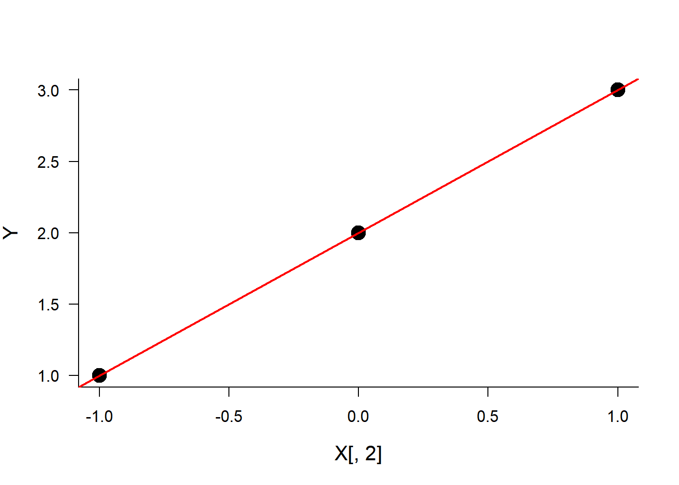
Obviously, the advantage of the matrix notation is its great generality. We can perform a linear regression of \(Y = 1,2,3\) against some covariate \(X = -1,0,1\) using the exact same code. We need only to set up the design matrix:

(X <- cbind(c(1,1,1), -1:1))

##      [,1] [,2]
## [1,]    1   -1
## [2,]    1    0
## [3,]    1    1

(H <- solve(t(X)%*%X)%*%t(X))

##            [,1]      [,2]      [,3]
## [1,]  0.3333333 0.3333333 0.3333333
## [2,] -0.5000000 0.0000000 0.5000000

(beta.hat <- H%*%Y)

##      [,1]
## [1,]    2
## [2,]    1

Y.hat <-X%*%beta.hat
(sigma.hat <- t(Y-Y.hat) %*% (Y - Y.hat) / (nrow(X) - ncol(X)))

##      [,1]
## [1,]    0

So the regression coefficients are \(\beta_0 = 2\) and \(\beta_1 = 1\), and \(\sigma^2 = 0\). Obviously, that’s correct, but if you need proof:

plot(X[,2],Y, cex=2, pch=19)
abline(t(beta.hat), col=2, lwd=2)