Wavelets
are literally "little waves", small oscillating waveforms that
begin from zero, swell to a maximum, and then quickly decay to
zero again. They can be contrasted to, for example, sine or
cosine waves, which go on "forever", repeating out to positive
and negative infinity. In the previous sections we have seen how
useful it is to use the Fourier Transform of a signal, which
expresses a signal as the sum of sine and cosine waves, allowing
such useful operations as convolution, deconvolution, and
Fourier filtering. But there is a down side to the Fourier
Transform; it covers the entire signal duration, giving only the
average frequency content. We saw in the previous section of the
Fourier transform that it is possible to use segmented or
time-resolved variations of the Fourier transform to overcome
this difficulty. But a more
sophisticated way to solve this limitation of Fourier analysis
is to use wavelets as a basis set for representing signals
rather than sine and cosine waves. Like sine waves, wavelets
can be stretched or compressed along their "x" or time axis to
cover different frequencies. But unlike sine waves, wavelets
can be translated along the time axis of a signal to
probe the time variations, because wavelets have a much
shorter duration compared to the signals they are used with.
Wavelets
were introduced by mathematicians and mathematical physicists in
the early years of the 20th century and the subsequent
development has been highly mathematical. Many of the treatments
of wavelets in the literature are aimed at the mathematical
aspects, which have been "worked out in excruciating detail"
(according to reference 80).
The value system of mathematics - rigorous proofs, exhaustive
exploration, assumption of mathematical background, and the need
for compact notation - make it difficult for the non-specialists.
Because of this, there are an unusually large number of "easy"
introductions to the subject (references 77 - 80) that
promise to soften the blow of mathematical abstraction. For that
reason, I will not repeat the mathematical details here. Rather, I
will attempt to show what you can accomplish using wavelets without understanding all
the underlying mathematics. I am particularly interested in
situations when the wavelets works better than the best available
conventional techniques, but also in situations where the
conventional techniques remain superior. A wavelet
transform (WT) is a decomposition of a signal into
a set of basis functions consisting of contractions, expansions,
and translations of a wavelet function (reference 83). It can be
computed by repeated convolution of the signal with the chosen
wavelet as the wavelet is translated across the time dimension, in
order to probe the time variation, and as the wavelet is stretched
or compressed, in order to probe different frequencies. Because
two dimensions are being probed, the result is naturally a 3D
surface (time-frequency-amplitude) that can be conveniently
displayed as a time-frequency contour plot with
different colors representing the amplitudes at that time and
frequency. Of course, one expects that such calculations will
require more complex algorithms and greater execution times. That
might have been a problem in the early days of computers, but with
modern fast processors and great memory capacity, it's unlikely to
be a problem.
Wavelets are
used for the visualization, analysis, compression, and denoising
of complex data. There are dozens of different wavelet shapes,
which by itself is a big difference from Fourier analysis. Three
of them, the Meyer, the Morlet and the Mexican hat, are mentioned
in the Wikipedia article
on waveletsand are
pictured above.
In
Matlab, the easiest way to access these
tools is to use the Wavelet
Toolbox, if that is included in your school or
company campus Matlab site license. This toolbox includes a
graphical user interface (GUI) for a Wavelet Analyzer, Signal
Multiresolution Analyzer, and a Wavelet Signal Denoiser, as well as
an extensive
collection
of command-line wavelet functions. Documentation is
available at https://www.mathworks.com/products/wavelet.html.
It's not absolutely necessary to have the Wavelet Toolbox, however.
Plenty of code has been published on the Internet in a variety of
languages. For example, Michael Cohen's paper in reference 82 includes
Matlab code that implements a Morlet wavelet using only the inbuilt
functions fft.m, ifft.m, and conv.m. I will use all of these
software approaches to describe the properties and applications of
wavelets to scientific measurement.
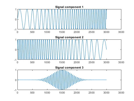
Wavelets are quite effective for visualizing complicated signals and
helping the scientist make sense of them. A good example is given in
reference
82, which describes a complex signal sampled at 1000 Hz and
consisting of three overlapping components that are initially
unknown to the experimenter. The separate components are shown in
the figure below: 1) a swept sine wave ('chirp') going from 5 Hz to
20 Hz, (2) another simultaneous swept sine wave ('chirp') going in
reverse, from 20 Hz to 5 Hz, and finally (3) a Gaussian-modulated 20
Hz sine wave that peaks in the center of the signal. This is clearly
an artificial construct, but it illustrates the power of
wavelets very well.
When these three added are up, the resulting time-domain waveform,
shown in the upper panel of the figure below (displayed
in iSignal.m),
is complicated and offers no hint of its underlying structure. The
conventional Fourier transform spectrum, shown in the lower panel,
shows only that the signal's frequency components are clustered
together into the middle frequency range, from about 4 Hz to 25 Hz.
In fact, the Fourier spectrum is misleading; it dips to zero at 12
Hz, suggesting that there might be only two components, one with
frequency components at a higher frequency range than the other,
with a small gap in between. But in fact there are actually three
components, two of them covering a wide frequency range and the
third one fixed at about 12 Hz.
In contrast, the wavelet-based signal analysis produces a time-frequency-amplitude contour
plot shown below, which is computed by the Matlab code in
the Michael Cohen's original paper (reference 82), helps to unravel the complexities,
showing all three components. In this display, yellow
corresponds to the greatest amplitudes and blue to the lowest. The
Gaussian-modulated 20 Hz component shows up clearly separated from
the rest, and the
two swept sine waves show up as a big X.
(There
is an interesting ambiguity concerning the two swept sine waves at
the point where they cross in frequency in the middle of the
signal; do they keep going in the same direction, forming an "X",
or do they both reverse direction, forming a "V" and its
reflection?The two
behaviors would result in the same final signal. The simplest
assumption would be the former).
Another example is closer to a typical scientific
application: digging a signal out of an excess of noise and
interference. The signal (top panel in the figure below) consists of
a pair of weak Gaussian peaks that are completely buried in a much
stronger interfering swept-frequency sine wave and random white
noise. The Fourier spectrum, observed here in the bottom panel,
again offers little hint of the underlying structure.
But the wavelet time-frequency-amplitude matrix shown above, using
the Morlet wavelet (script
and Morlet
wavelet function) is more revealing. The big yellow
diagonal stripe corresponds to the swept sine wave interference, but
you can also see two weaker green blobs near the bottom at low
frequencies, near time data points=0.4 and 1 (x104).
On the basis of that observation, you would be justified to look
more closely in that region and to perform smoothingor curve-fitting, which will
reveal the two Gaussian peaks there. (You can compare this graphic
to the segmented Fourier
spectrum display for this signal shown, which is cruder but
displays similar information; the wavelet is clearly a finer-grained
tool than my segmented Fourier Transform function).
In the context of wavelets, "denoising" means reducing the noise as
much as possible without distorting the signal. Denoising makes use
of the time-frequency-amplitude matrix created by the wavelet
transform. It's based on the assumption that the undesired noise
will be separated from the desired signal by their frequency ranges.
Most commonly in scientific measurements, the desired signal
components are located at relatively low frequencies and the noise
is mostly at high frequencies. The process is controlled both by the
selection of wavelet type and by a positive integer number called
the wavelet "level"; the higher the level, the lower is the
frequency divider between signal and noise. (To that extent, the
wavelet level is similar to the effect of the smooth width of a
smoothing operation).
Again, Matlab's Wavelet Toolbox provides some useful tools. First,
there is the GUI app called the "Wavelet Signal Denoiser". The
selection of the wavelet type and level are all selectable manually
in the Wavelet Signal Denoiser app. I used that app to analyze the
"buried peaks" signal as previously, using the "sym4" wavelet at a
relatively high level of 11, because lower levels allow too much of
the interfering swept sine wave to come through and higher levels
would damp out the Gaussian peaks too much. The "Approximation"
result (the dotted line) is the low-frequency information in the
data, and you can clearly see that this is a "denoised" version of
the original signal (shown in blue).The two bumps at sample numbers 5000 and 10000 are the two
Gaussian peaks.
So both the sym4 wavelet in the Denoiser and the Morlet wavelet's
time-frequency-amplitude matrix give evidence of the hidden Gaussian
peaks, but displayed in a different way.
In addition to the GUI app, there is also a command-line function
denioising function called "wdenoise.m" (syntax:DenoisedData=wdenoise(noisydata,level, ...).
The
selection of the wavelet type and level are set by including
optional input arguments to this function.
The advantage of using a function, compared to the GUI app,
is that it's possible to write scripts that quickly and
automatically compare many different wavelet settings, that compare
the results to several conventional noise reduction methods, or that
automate the batch processing of large numbers of stored data sets
(see Batch processing).
For example, the question of the optimal selection of wavelet level
can be answered by the script OptimizationOfWaveletLevel3peaks.m,
which creates a simulated signal consisting of three noisy
unit-height Gaussian peaks with different peak widths, with added
white noise. The upper panel in this figure shows the underlying
pure noiseless Gaussians (blue line) and the red line shows those
peaks with white noise added. The lower panel shows the results of
wavelet denoising the noisy signal, in red, compared to the
underlying pure Gaussians in blue.
The script uses the wdenoise.m function to denoise them with the
"coiflet" wavelet for each level from 1 to 11, measuring three
quantities for each denoised signal: (a) the height of the peaks,
(b) the signal-to-noise ratio improvement, and (c) the closeness to
the noiseless underlying signal, as shown in the three plots below.
We can see from these plots that a level of about 7 is optimum
in this case; above 7, the signal-to-noise ratio (center graph)
continues to increase but the results are unreliable and tend to
scatter around too much. Changing to Lorentzian peaks (line 28 of
the script) yields similar results.
The script WaveletsComparison.m
compares five different wavelet types on the same
signal: BlockJS, bior5.5, coif2, sym8, and db4, all at level 12
(graphic).
The
results are similar but the sym8 has a slight edge. For most
smooth peak shapes with additive white noise, the different
wavelets perform similarly. For signals with high-frequency
weighted noise, the bior5.5
wavelet works better than the others (script;
graphic).
For
square pulses, however, the Haar
wavelet
is clearly superior.
Another
script
compares five different non-wavelet smoothing techniques and two
different wavelets, all using the same simulated signal consisting
of two Gaussian peaks with a 50-fold difference in peak width,
in order to test for adaptability to peak width variation. For each
method, the percent errors in the peak height, width, and area are
measured, as well as the "residual", which is the difference between
the underlying noiseless signal and the denoised (or smoothed) noisy
signal. This illustrates a significant advantage that wavelet
denoising has over smoothing; it adapts much better to changes in
peak width. A summary of typical results is shown in this table and
this graphic. (Peak 1 is the narrow peak and peak 2 is 50 times
wider).
The "Residuals"
are the percent differences between the underlying noiseless
signal and the signal with random noise after denoising; it
accounts for both residual noise left in the signal and
distortion of the signal shape. As you
can see, the "coif" wavelet (marked in red) comes out ahead by
most measures. This illustrates the most significant practical
advantages of wavelet denoising: (1) it gives results that are
at least as good, and often better, than conventional
smoothing methods, (2) it's easier to use because it
automatically adapts to different peak widths; and (3) it's
easier to optimize because usually only the level setting
makes much difference.
However,
there are a few situations where conventional methods are
better. For example, in calculating the second derivatives of
noisy peaks of variable width, a segmented Gaussian-weighted
smooth gives a signal-to-noise
ratio better than that of a wavelet denoise (script;
graphic),
especially
if the signal-to-noise ratio is poor (graphic),
presumably
because the frequency spectrum of the noise is so strongly
high-frequency weighted. Also, wavelet denoising does
not work well if the amplitude of the noise is proportional to the
signal amplitude rather than constant (script;
graphic).
Sometimes,
if the original signal-to-ratio is very poor, wavelet
denoising produces narrow spike artifacts in the denoised
signals, even when soft
thresholding is used. These are special cases;
there are many more situations where the wavelet denoise is
really the method of choice.
Updated March, 2024 This page is part of "A Pragmatic
Introduction to Signal Processing", created and
maintained by Prof. Tom O'Haver, Department of Chemistry and
Biochemistry, The University of Maryland at College Park. Comments,
suggestions and questions should be directed to Prof. O'Haver at toh@umd.edu.
Unique visits since May 17, 2008:


