Load data and packages:

load("../data/SMBT.rda")
pcks <- c("magrittr", "plyr", "ggplot2", "nlme")
a <- sapply(pcks, require, character = TRUE)

Goal

Here, we are interested in analyzing the pairwise similarity of the communities, which can be very diverse and variable (though often dominated by acne, unsurprisingly). As an example, here is one individual’s species composition along a single arm transect:

  require(gplots)
  par(mfrow = c(1,2), mar = c(4,4,2,0), tck = -0.01, mgp = c(1.5,.5,0), cex.axis = 0.75)
  ax1 <- subset(SMBT, Person == 12 & Transect == "ax")
  myTaxa <- unique(ax1$Taxon[ax1$Relative_Abundance > 0])
  n = length(myTaxa)
  palette(rich.colors(n))
  with(ax1, barplot(table(as.character(Relative_Abundance), Location), col = 1:n, bor = NA, space = .1))
  plot.new()
  par(mar = c(0,0,0,0))
  legend("left", legend = myTaxa, fill = 1:length(myTaxa), cex=0.5, ncol = 4, bty = "l")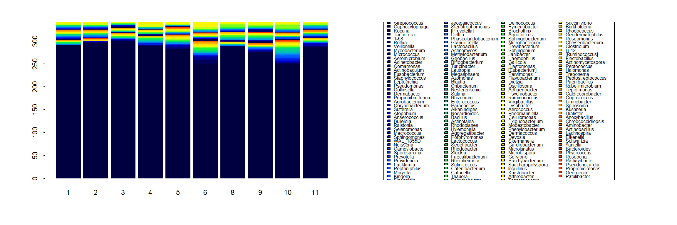

With so many taxa, it is very difficult to pick out strong individual taxa. Our goal here is to quantify how similar the communities are across locations.

Bray-Curtis Similarity

The Bray-Curtis similarity index compares the relative abundances of a community across two locations. For sites \(i\) and \(j\), with vector of abundance \({\bf a}\) of length \(n\) indexed over \(k\), this quantity is given by: \[ BC_{ij} = 1 - {\sum_{k=1}^n |a_{i,k} - a_{j,k}| \over \sum_{k = 1}^n (a_{i,k} + a_{j,k})}\]

A value of 0 indicates total dissimilarity, a value of 1 indicates total similarity - i.e.\(BC_{i,i} = 1\).

Here is a functions that compute the Bray-Curtis similarity:

getBrayCurtis <- function(A1, A2){
    A.12 <- merge(A1, A2, by = "Taxon", all = TRUE) 
    names(A.12) <- c("Taxon", "A1", "A2")
    with(A.12, 1 - sum(abs(A1 - A2))/sum(A1 + A2))
}

and a function that fills out a matrix across locations with BCS.

buildBrayCurtisMatrix <- function(data){
  locs <- unique(data$Location)
  n.locs <- length(locs)
  BC.matrix <- matrix(NA, nrow = n.locs, ncol = n.locs)
  row.names(BC.matrix) <- locs
  colnames(BC.matrix) <- locs
  
  for(i in 1:n.locs) for(j in 1:n.locs){
    A1 <- subset(data, Location == locs[i])[,c("Taxon","Relative_Abundance")]
    A2 <- subset(data, Location == locs[j])[,c("Taxon","Relative_Abundance")]
    BC.matrix[i,j] <- getBrayCurtis(A1, A2)
  }
  return(BC.matrix)
}

Here is a visualization of the pairwise Bray-Curtis similarity across Person 1’s Arm-X transect:

AX <- subset(SMBT, Transect == "ax")
IDs <- unique(AX$Person)

m <- buildBrayCurtisMatrix(subset(AX, Person == "1"))
require(fields)
par(mgp = c(1.5,.5,0), tck = 0.01, las = 1, cex.axis = 0.8)
n <- as.numeric(row.names(m))
image.plot(n, n, m, asp=1, ylab = "", xlab = "",
           main= "Bray-Curtis distance matrix", bty="l'")
title(sub = "Person 1", cex.sub=1.25)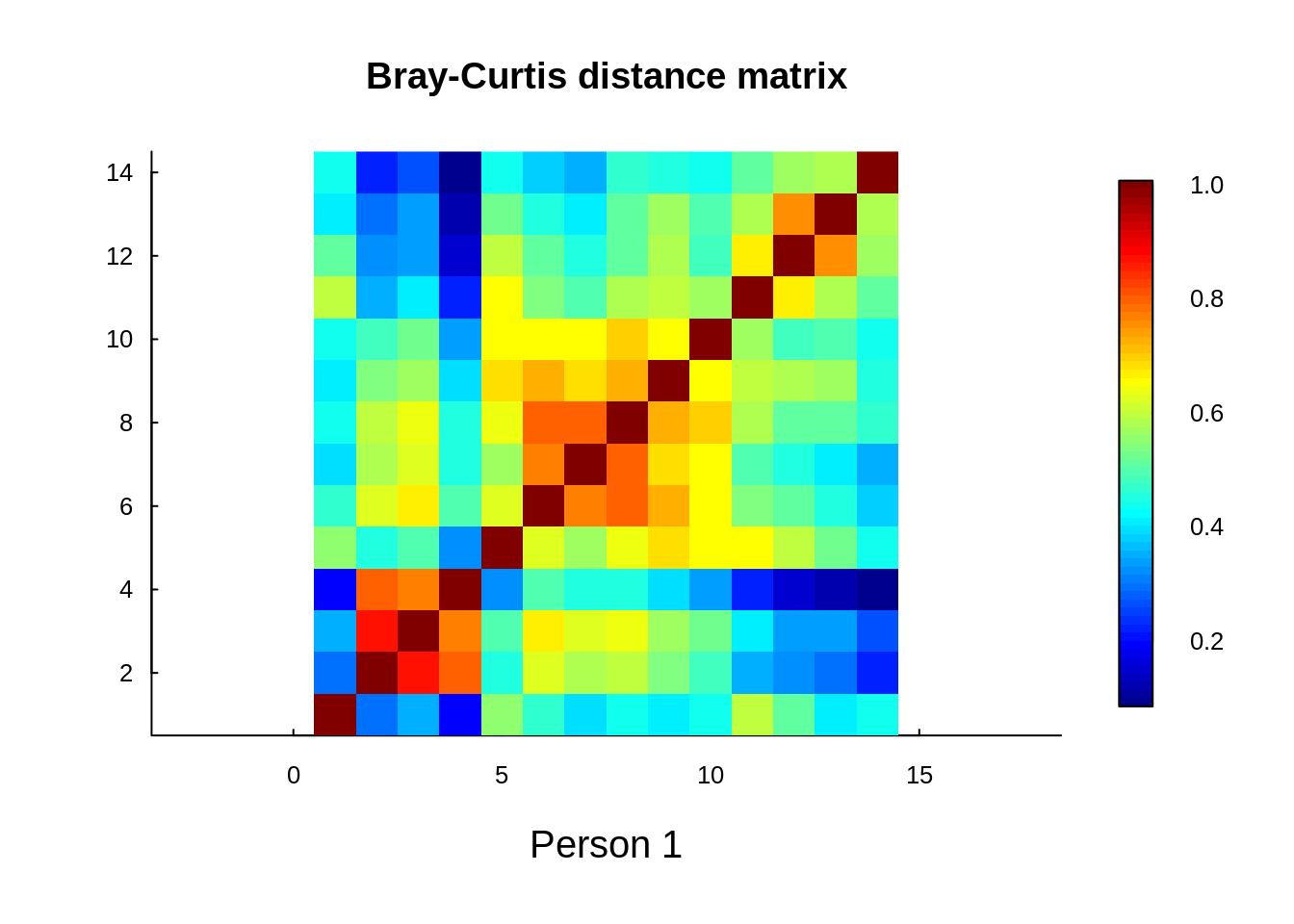

We hypothesize that:

There is spatial correlation in community similarity across transects

That some of that variability can be explained by:

absolute magnitude of environmental variables

relative difference of environmental variables

Computing BCI for all data

The following code computes all the pairwise BCI’s for each person and each transect, and saves the resulting computations into a file for ready access later.

# compute all of them 
require(plyr); require(magrittr)
E <- c("Moisture", "Temperature", "pH", "Sebum")
AllMatrices <- dlply(SMBT, c("Person", "Transect"), 
                     function(df){ 
                       p <- df$Person[1]
                       t <- df$Transect[1]
                       E <- ddply(df, "Location", summarize, 
                             Sebum = mean(Sebum), 
                             Moisture = mean(Moisture), 
                             Temperature = mean(Temperature),
                             pH = mean(pH)) %>% na.omit
                        
                       list(Person = p, 
                            Transect = t, 
                            BC.matrix = buildBrayCurtisMatrix(df),
                            Environment = E
                            )
                       })
save(AllMatrices, file = "../data/AllMatrices.rda")

This code generates a data frame with all of the pair-wise BCI computations, together with the environmental covariate measures:

load(file = "../data/AllMatrices.rda")

# Generate complete processed distance data frame

makeDF <- function(l){
  locs <- as.numeric(row.names(l$BC.matrix))
  
  M <- l$BC.matrix
  D <- abs(outer(locs, locs, "-"))
  loc1 <- outer(locs, locs, function(x,y) x)
  loc2 <- outer(locs, locs, function(x,y) y)
  
  upper <- upper.tri(M)
  BC.df <- data.frame(Person = l$Person, Transect = l$Transect,
             Loc1  = loc1[upper], Loc2 = loc2[upper],
             Distance =  D[upper], BC = M[upper])
  
  # get dEnvironment
  
  E <- l$Environment
  upper <- upper.tri(matrix(0, nrow(E), nrow(E)))
   
  dE.df <- with(E, data.frame(
     Loc1 = as.vector(outer(Location, Location, function(x,y) x)[upper]),
     Loc2 = as.vector(outer(Location, Location, function(x,y) y)[upper]),
     
     dSebum = as.vector(outer(Sebum, Sebum, "-")[upper]),
     dMoisture = as.vector(outer(Moisture, Moisture, "-")[upper]),
     dTemperature = as.vector(outer(Temperature, Temperature, "-")[upper]),
     dpH = as.vector(outer(pH, pH, "-")[upper]))
   )
  
  merge(dE.df, BC.df, all=TRUE)
}

Transect.df <- ldply(AllMatrices, makeDF)

# get average values of covariates across individuals, and merge

Covar.means <- ddply(SMBT, c("Person", "Transect"), summarize, 
                     Sebum.mean = mean(Sebum, na.rm=TRUE), 
                     Temperature.mean = mean(Temperature, na.rm=TRUE), 
                     Moisture.mean = mean(Moisture, na.rm=TRUE), 
                     pH.mean = mean(pH, na.rm=TRUE)) 

Transect.df <- merge(Transect.df, Covar.means, all= TRUE)
save(Transect.df, file = "../data/Transect.df.rda")

Plots of all the data

Note - the Y-axes are on a log scale.

(Click on the tabs to see the different plots!)

Arm X

ggplotAll(subset(Transect.df, Transect == "ax"), "Arm X")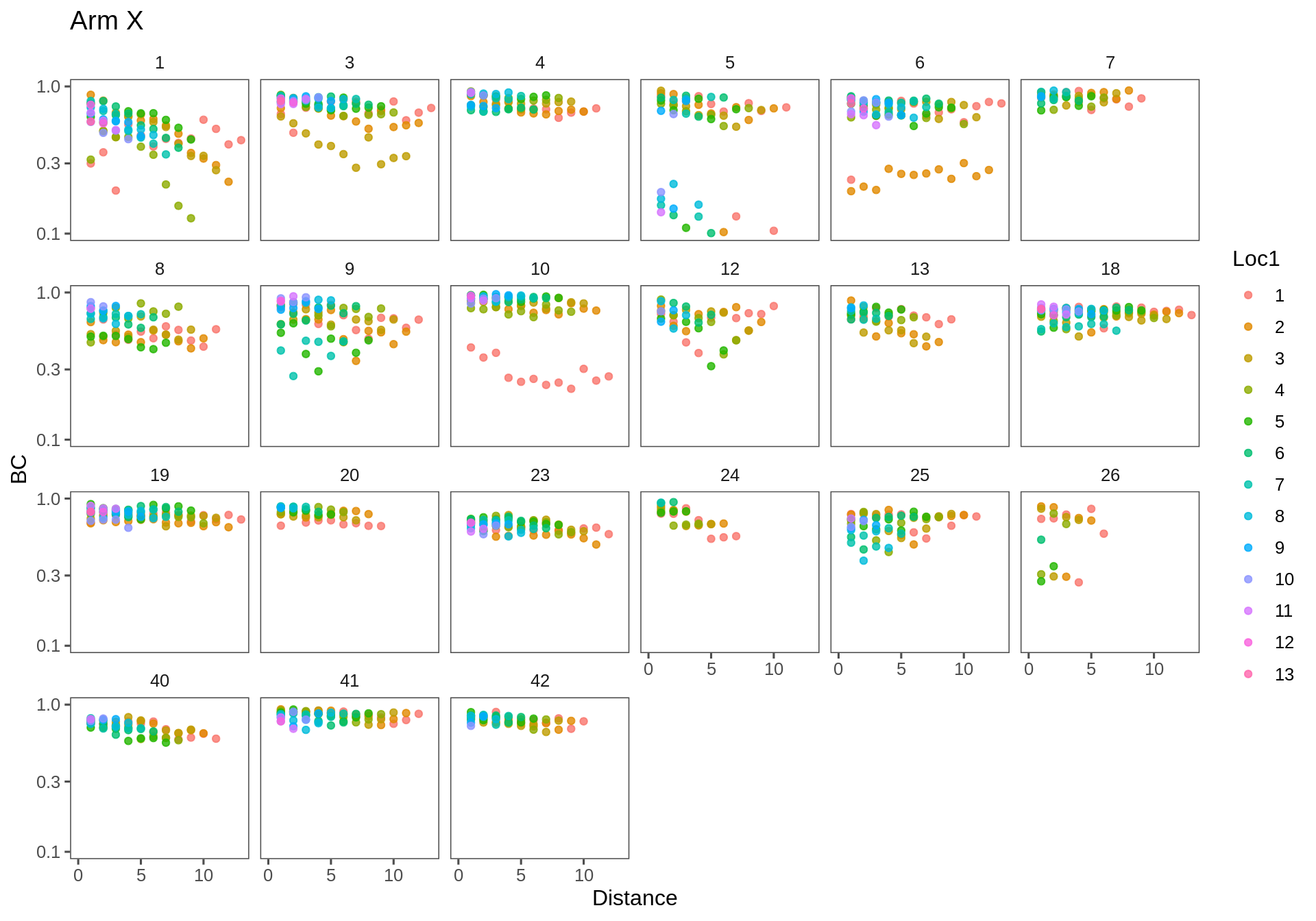

Arm Y

ggplotAll(subset(Transect.df, Transect == "ay"), "Arm Y", xmax = 8)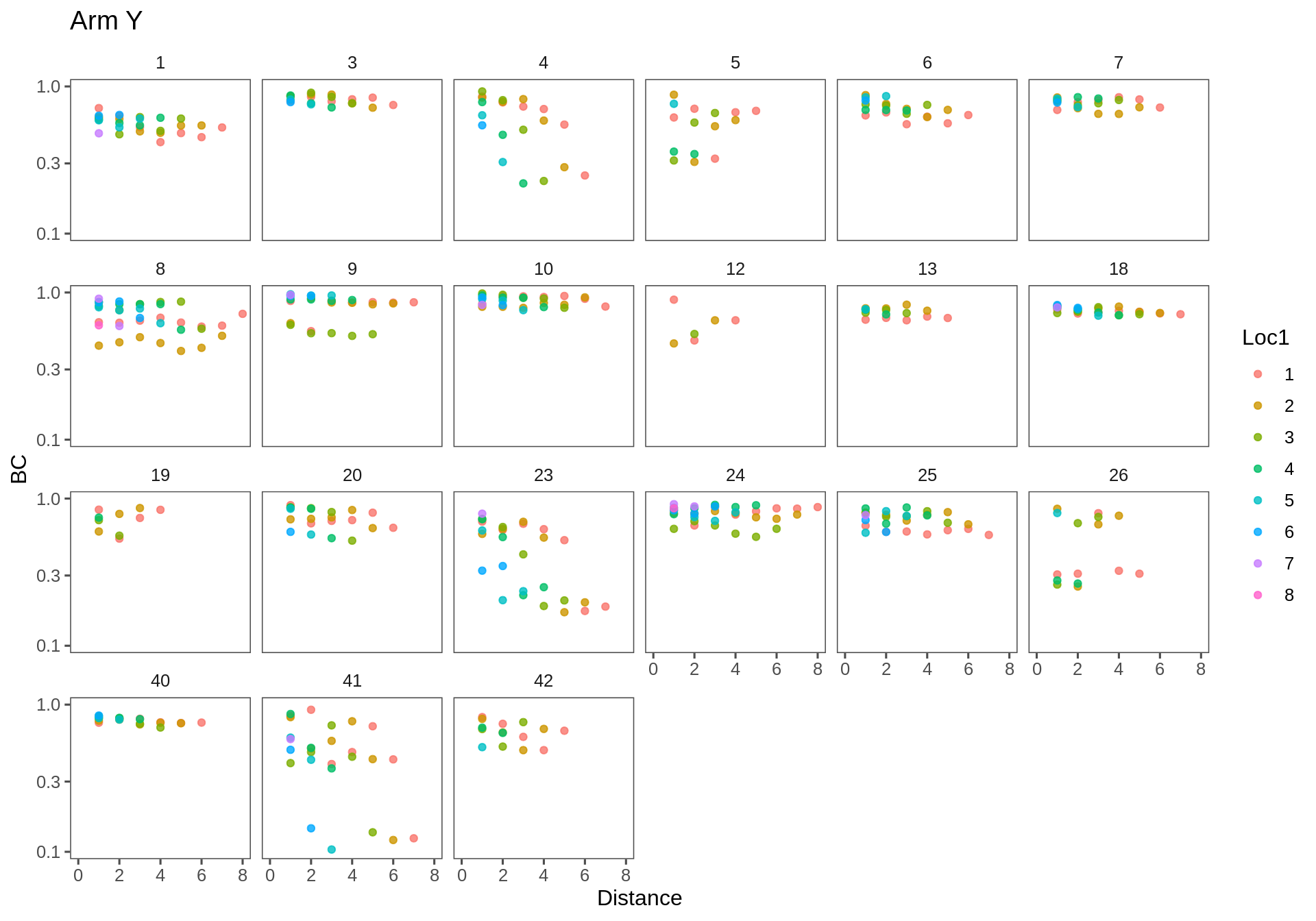

Face X

ggplotAll(subset(Transect.df, Transect == "fx"), "Face X", ymin = 0.4, xmax = 8)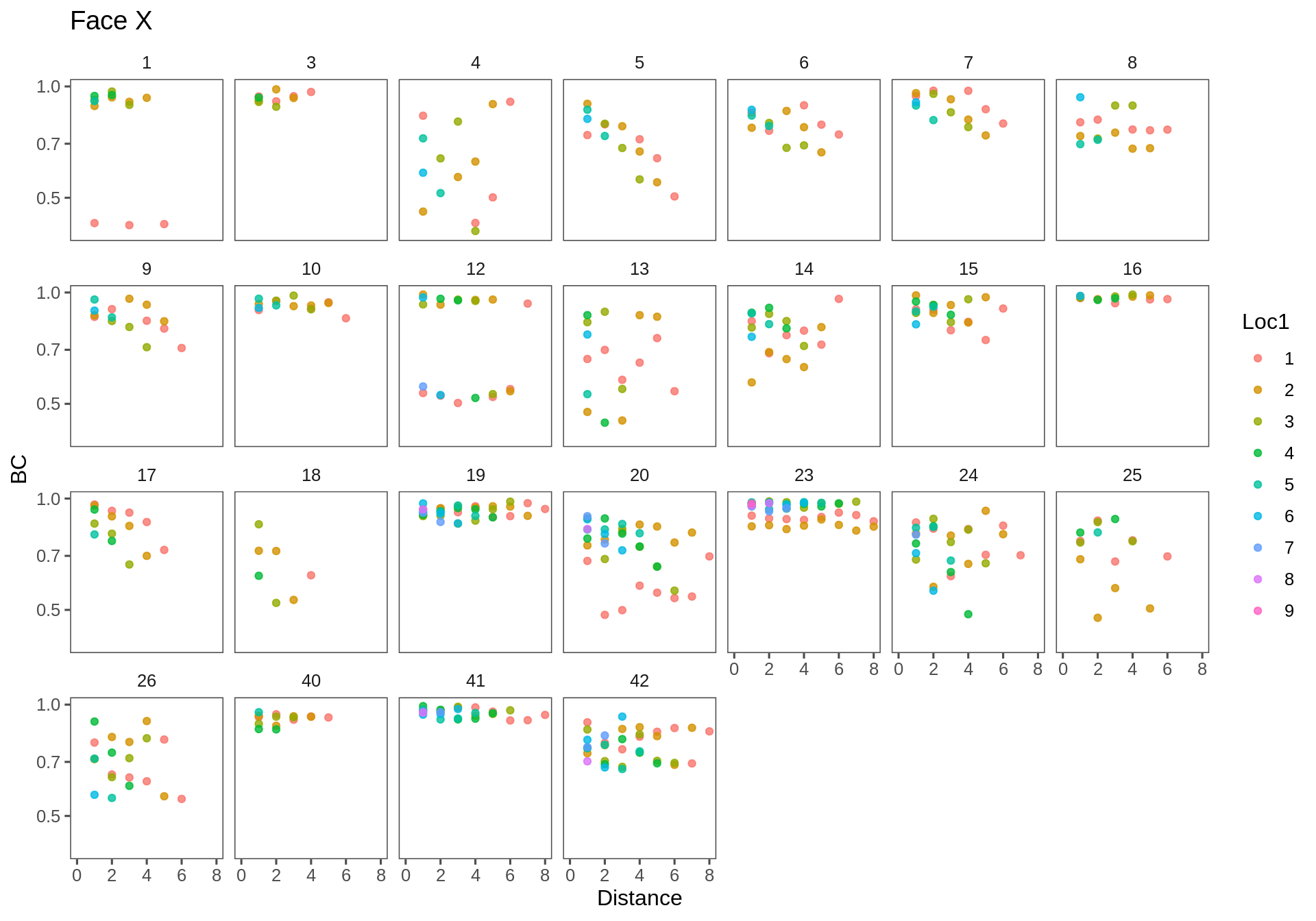

Observations

The general trend is of decrease, as expected. One would expect the intercept to be strictly 1 (the similarity is always 1 at distance 0) - though many clouds appear to have a lower intercept [e.g. AX-23]. Some similarities across distances are extremely high (e.g. AX-4,7,10,19; FX-19,23). Some linear effects are really strong and steep (e.g. AX-24, FX-5). One item of concertn is that there are several outlying sets - if one site is very different from the rest (e.g. in AX-5,6; AY-26; FX-12) - then a whole bunch of points will drag the overall similarity way down.

Modelling

A proposed model:

\[\log(BC_{ij}) = \beta_0 + \beta_d D_{ij} + \beta_e \Delta{\bf E}_{ij} + \epsilon\]

Where \(D_{ij}\) is the distance between locations (the greater the distance, the lower the similarity), and \(\Delta{{\bf E}}\) is the difference in the (vector) of environmental covariates [possibly normalized by the absolute value, i.e. percent change]. Note, the intercept \(\beta_0\) in this model could be fixed to 0, since at \(D_{ij} = 0\) and \(\Delta{\bf E}_{ij} = 0\), the similarity is 1, i.e. log-intercept is 0.

This model is for a particular person - for which there is not very much data. But a mixed effects model can be fit for the entire population, in which the estimated parameters are modeled as a random effect, i.e.:

\(\beta_k \sim {\cal N}(\mu_\beta, \sigma_\beta)\)

which is a robust and tractable model.

One advantage of this model is that - given some sort of distance metric - we can combine both the x and y transects for the arm and face. Also it is easy to fit. Also, it combines all possible pairs, so even with 10 samples along a transect, that are still 45 pairs.

We will fit the models systematically:

First: individual models with no covariates (with and without intercept)
Second: individual models with covariates - only where measured
Third: individual models with interpolated covariates
Finally: mixed effects models

ggplotWithPrediction <- function(data, model = NULL, ...){
  
  data <- mutate(data, Loc1 = factor(Loc1))
  
  if(!is.null(model)){
    prediction <- predict(model, newdata = data, se=TRUE)
    data <- mutate(data, 
      y.hat = exp(prediction$fit),
      y.low = exp(prediction$fit - 2*prediction$se),
      y.high = exp(prediction$fit + 2*prediction$se))
  }
  
  baseplot <- ggplotAll(data, ...)
  fullplot <- baseplot + 
        geom_line(data = data, 
                  aes(x = Distance, y = y.hat), 
                  col="darkred", lwd = 1, alpha = 0.5) + 
        geom_line(data = data, 
                  aes(x = Distance, y = y.high), 
                  col="red", lwd = .5, alpha=0.5) + 
        geom_line(data = data, 
                  aes(x = Distance, y = y.low), 
                  col="red", lwd = .5, alpha = 0.5) + 
    theme(legend.position="none")
  print(fullplot)
}

fitModel <- function(df, f){
    mylm <- lm(f, data = df)
    prediction <- predict(mylm, newdata = df, se=TRUE)
    mutate(df, 
      y.hat = exp(prediction$fit),
      y.low = exp(prediction$fit - 2*prediction$se),
      y.high = exp(prediction$fit + 2*prediction$se))
}

Individual model, no covariates, no intercept

The no-intercept model makes sense, but it is not, in fact, very good as can be seen in the figures below.

T.lm1 <- ddply(Transect.df, c("Transect", "Person"), fitModel, f = formula(log(BC)~Distance - 1))

Arm X

ggplotWithPrediction(subset(T.lm1, Transect == "ax"),  
                     title = "Arm X - linear model no intercept", log=FALSE)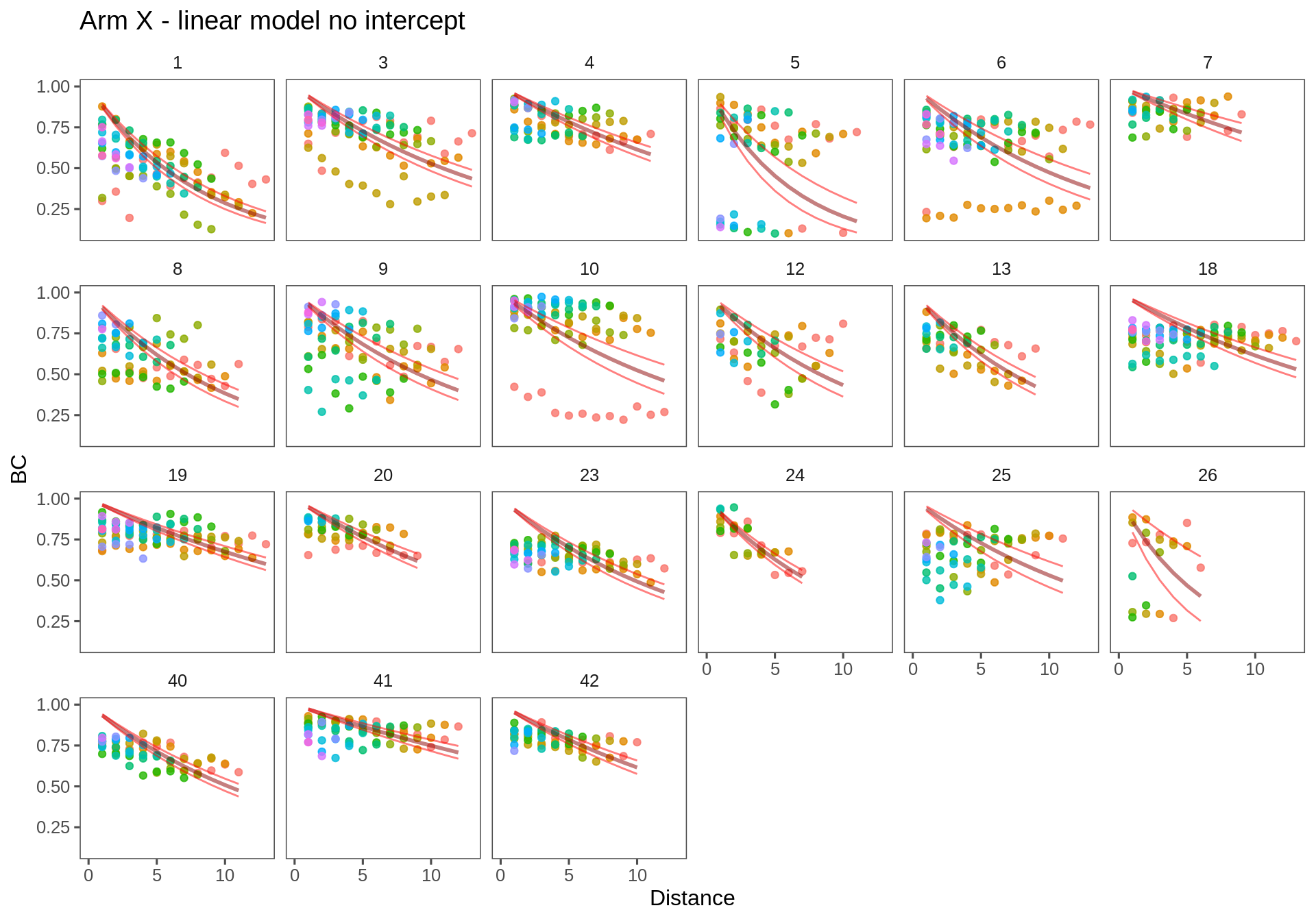

Arm Y

ggplotWithPrediction(subset(T.lm1, Transect == "ay"), 
                     title = "Arm Y - linear model no intercept",
                     xmax = 8)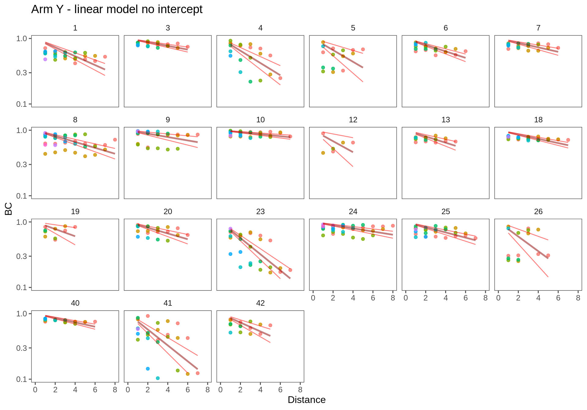

Face X

ggplotWithPrediction(subset(T.lm1, Transect == "fx"), 
                     title = "Face X - linear model no intercept", 
                     ymin = 0.4, xmax = 8)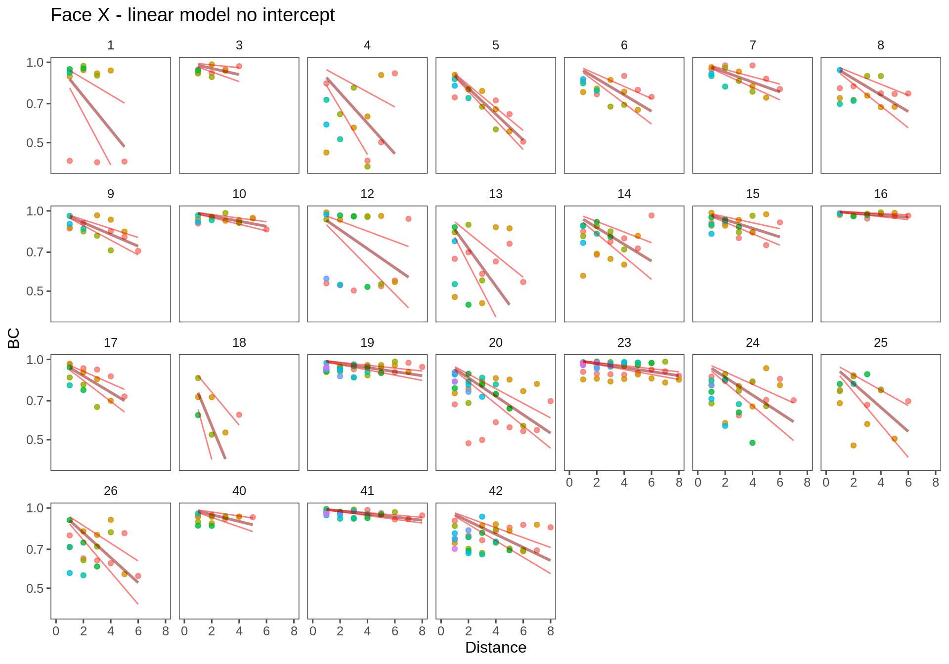

Individual model, no covariates with intercept

Individually, these fits look much better / more informative. Here, the intercepts can be interpreted as an overall measure of similarity. Maybe even, more specifically, use the mean value (i.e. the point estimate the half-max distance) as a measure of the overall similarity.

One imporant issue: OUTLYING POINTS! Honestly, I would be tempted to just knock out those - there are relatively few EXTREMELY dissimilar locations, but they throw a lot off.

T.lm2 <- ddply(Transect.df, c("Transect", "Person"), fitModel, f = formula(log(BC)~Distance))

Arm X

ggplotWithPrediction(subset(T.lm2, Transect == "ax"), 
                     title = "Arm X - linear model", log=FALSE)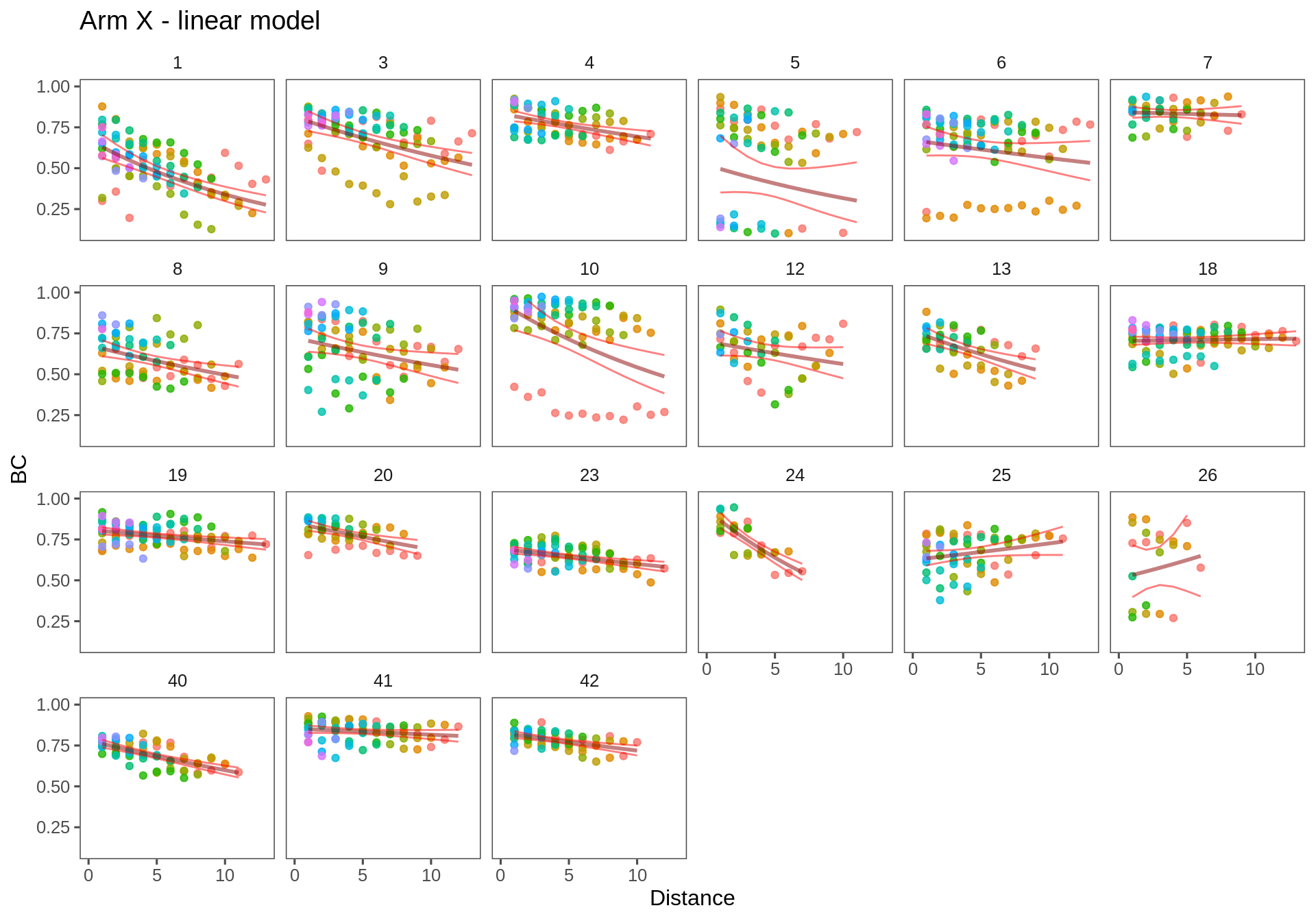

Arm Y

ggplotWithPrediction(subset(T.lm2, Transect == "ay"), 
                     title = "Arm Y - linear model",
                     xmax = 8, log = FALSE)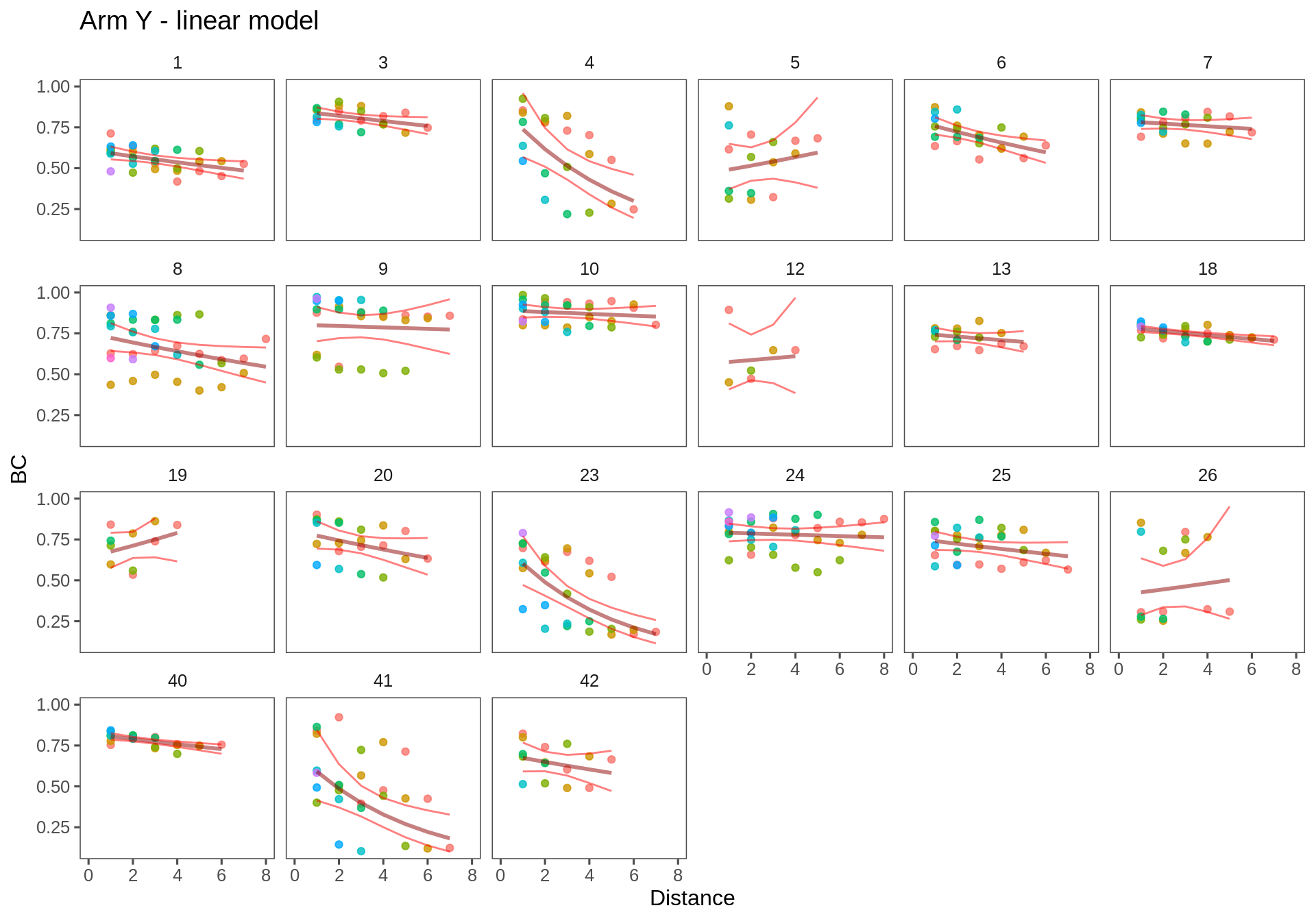

Face X

ggplotWithPrediction(subset(T.lm2, Transect == "fx"), 
                     title = "Face X - linear model", 
                     ymin = 0.4, xmax = 8, log = FALSE)

Coefficients across covariates

reportLM2coefs <- function(df){
    mylm <- lm(log(BC)~I(Distance-mean(Distance)), data = df)
    coefs <- summary(mylm)$coef[cbind(c(1,1,1,2,2,2),c(1,2,4,1,2,4))] 
    names(coefs) <- c("alpha", "alpha.se", "alpha.pvalue", "beta", "beta.se", "beta.pvalue")
    data.frame(t(coefs))
}

covars <- c("Sebum", "Temperature", "pH", "Moisture")

T.coefs <- ddply(Transect.df, c("Person","Transect", paste0(covars,".mean")), reportLM2coefs) %>% mutate(BC.mean = exp(alpha))

grid_arrange_shared_legend <- function(...) {
    plots <- list(...)
    g <- ggplotGrob(plots[[1]] + theme(legend.position="bottom"))$grobs
    legend <- g[[which(sapply(g, function(x) x$name) == "guide-box")]]
    lheight <- sum(legend$height)
    grid.arrange(
        do.call(arrangeGrob, lapply(plots, function(x)
            x + theme(legend.position="none"))),
        legend,
        ncol = 1,
        heights = unit.c(unit(1, "npc") - lheight, lheight))
}

Question: How many individuals have “significant spatial organization” (per body site). Significant slope with distance.

ddply(T.coefs, "Transect", summarize, P.signif = sum(beta.pvalue < 0.05)/length(beta.pvalue))

Arm-X is consistently the most spatially structured of the transects.

Alpha-Covariate plot

Plot of average (log(MEAN)) similarity against covariates:

require(gridExtra)
g.Sebum = ggplot(T.coefs, aes(Sebum.mean, BC.mean, col = Transect)) + geom_point() + stat_smooth(method = "lm") + theme_few()
g.Temperature = ggplot(T.coefs, aes(Temperature.mean, BC.mean, col = Transect)) + geom_point() + stat_smooth(method = "lm") + theme_few()
g.pH = ggplot(T.coefs, aes(pH.mean, BC.mean, col = Transect)) + geom_point() + stat_smooth(method = "lm") + theme_few()
g.Moisture = ggplot(T.coefs, aes(Moisture.mean, BC.mean, col = Transect)) + geom_point() + stat_smooth(method = "lm") + theme_few()

grid_arrange_shared_legend(g.Sebum, g.Temperature, g.pH, g.Moisture)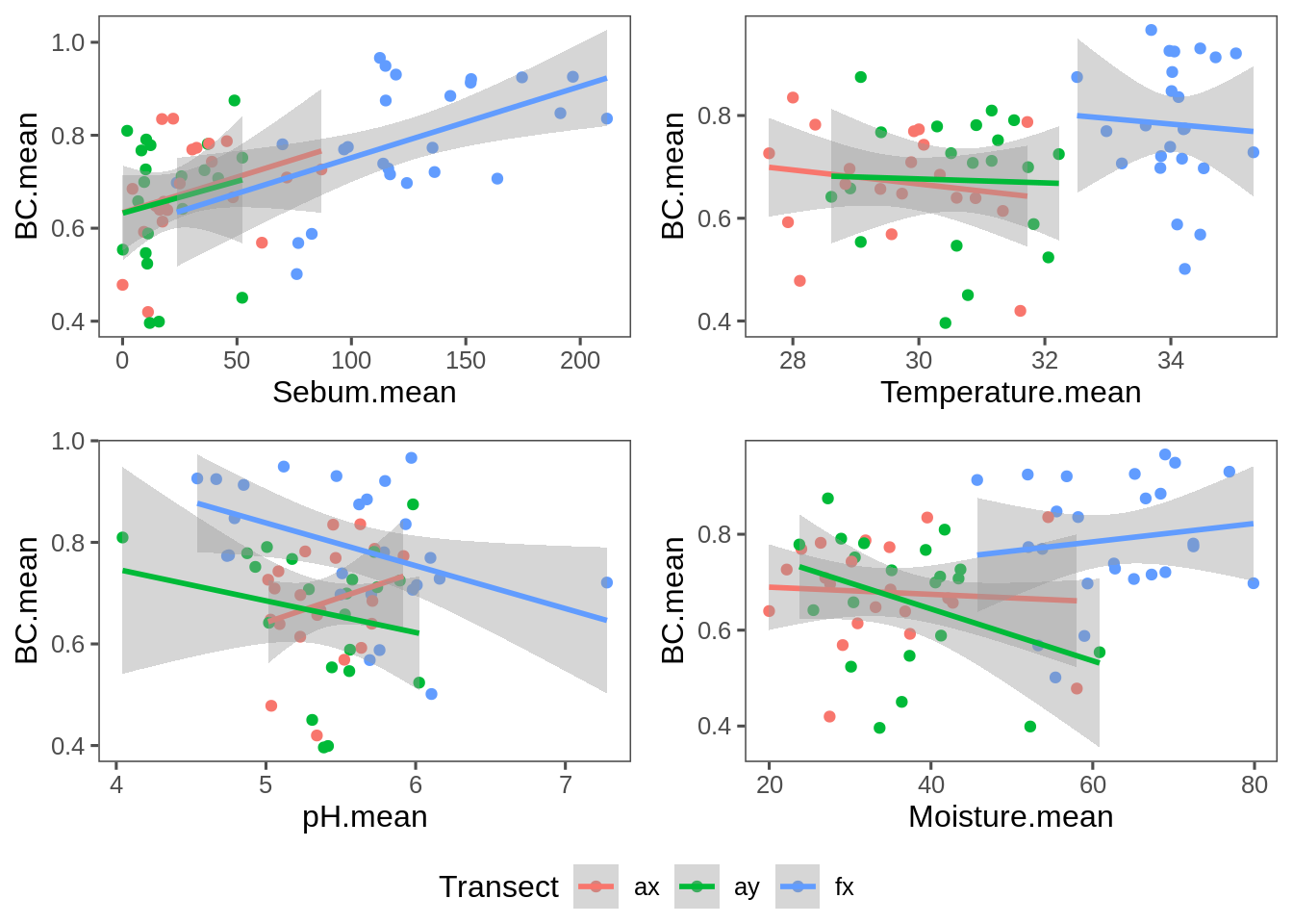

Very consistent: High sebum means higher similarity across all transects.

Statistical tests:

summarize.meta.BCmean <- function(df){
  results <- data.frame(NULL)
  for(covar in paste0(covars, ".mean")){
    mylm <- lm(df[,"BC.mean"] ~ scale(df[,covar]), data = df)
    results <- rbind(results, data.frame(t(summary(mylm)$coef[cbind(c(2,2), c(1,4))])) %>% rename(c("X1" = "beta", "X2" = "p.value")) %>% mutate(covar = covar))
  }
  results
}

ddply(T.coefs, "Transect", summarize.meta.BCmean) %>% subset(p.value < 0.1)

Only in faces is the slope coefficient significant for Sebum and pH

Faces are generally more similar across transects:

require(nlme)
lme(BC.mean~Transect-1, random = ~1|Person, data = T.coefs) %>% summary

## Linear mixed-effects model fit by REML
##  Data: T.coefs 
##         AIC       BIC   logLik
##   -67.71068 -56.91626 38.85534
## 
## Random effects:
##  Formula: ~1 | Person
##         (Intercept)  Residual
## StdDev:  0.05395599 0.1121821
## 
## Fixed effects: BC.mean ~ Transect - 1 
##                Value  Std.Error DF  t-value p-value
## Transectax 0.6820332 0.02708766 40 25.17874       0
## Transectay 0.6637860 0.02708766 40 24.50511       0
## Transectfx 0.7893827 0.02489665 40 31.70638       0
##  Correlation: 
##            Trnsctx Trnscty
## Transectay 0.183          
## Transectfx 0.173   0.173  
## 
## Standardized Within-Group Residuals:
##         Min          Q1         Med          Q3         Max 
## -2.41938194 -0.49276302 -0.02905331  0.75607929  1.41748361 
## 
## Number of Observations: 67
## Number of Groups: 25

boxplot(BC.mean~Transect, data = T.coefs)

Beta-Covariate plot

Plot of slope similarity (spatial correlation measure) against covariates:

g.Sebum = ggplot(T.coefs, aes(Sebum.mean, beta, col = Transect)) + geom_point() + stat_smooth(method = "lm") + theme_few()
g.Temperature = ggplot(T.coefs, aes(Temperature.mean, beta, col = Transect)) + geom_point() + stat_smooth(method = "lm") + theme_few()
g.pH = ggplot(T.coefs, aes(pH.mean, beta, col = Transect)) + geom_point() + stat_smooth(method = "lm") + theme_few()
g.Moisture = ggplot(T.coefs, aes(Moisture.mean, beta, col = Transect)) + geom_point() + stat_smooth(method = "lm") + theme_few()

grid_arrange_shared_legend(g.Sebum, g.Temperature, g.pH, g.Moisture)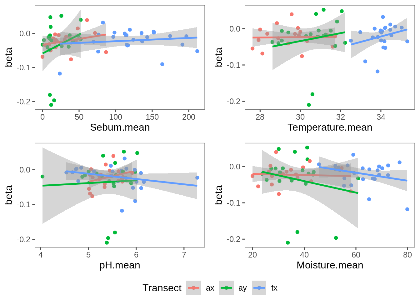

None of these are significant. The following code tabulates the relationships:

summarize.meta.Beta <- function(df){
  results <- data.frame(NULL)
  for(covar in paste0(covars, ".mean")){
    mylm <- lm(df[,"beta"] ~ scale(df[,covar]), data = df)
    results <- rbind(results, data.frame(t(summary(mylm)$coef[cbind(c(2,2), c(1,4))])) %>% rename(c("X1" = "beta.beta", "X2" = "p-value")) %>% mutate(covar = covar))
  }
  results
}

ddply(T.coefs, "Transect", summarize.meta.Beta) %>% rename(c("p-value" = "p.value")) %>% arrange(p.value)

Furthermore, there are no significant differences in that spatial structure across transects:

lme(beta~Transect-1, random = ~1|Person, data = T.coefs) %>% summary

## Linear mixed-effects model fit by REML
##  Data: T.coefs 
##         AIC       BIC   logLik
##   -188.9211 -178.1267 99.46057
## 
## Random effects:
##  Formula: ~1 | Person
##         (Intercept)   Residual
## StdDev: 1.42879e-06 0.04756167
## 
## Fixed effects: beta ~ Transect - 1 
##                  Value   Std.Error DF   t-value p-value
## Transectax -0.02265200 0.010378808 40 -2.182524  0.0350
## Transectay -0.03542515 0.010378808 40 -3.413220  0.0015
## Transectfx -0.02019273 0.009512334 40 -2.122794  0.0400
##  Correlation: 
##            Trnsctx Trnscty
## Transectay 0              
## Transectfx 0       0      
## 
## Standardized Within-Group Residuals:
##        Min         Q1        Med         Q3        Max 
## -3.6647134 -0.2497056  0.1805346  0.4416407  1.8395825 
## 
## Number of Observations: 67
## Number of Groups: 25

lme(beta~Transect, random = ~1|Person, data = T.coefs) %>% anova

Difference Analysis

Relative change vs. BC

Here, we’re looking at the relationship between the BC and the relative change in the covariate across sites.

T2 <- na.omit(Transect.df)
T2 <- ddply(T2, c("Person","Transect"), 
  function(df){
    me <- df[,c("Loc1", "Loc2")]
    ls <- sort(unique(as.vector(as.matrix(me))))
    for(i in 1:3)
      me[me == ls[i]] <- i
    df[,c("Loc1", "Loc2")] <- me
    df$Distance <- abs(df$Loc2 - df$Loc1)
    df$Sebum.mono <- df$dSebum[3]*df$dSebum[1] > 0
    df$Temperature.mono <- df$dTemperature[3]*df$dTemperature[1] > 0
    df$Moisture.mono <- df$dMoisture[3]*df$dMoisture[1] > 0
    df$pH.mono <- df$dpH[3]*df$dpH[1] > 0
    df
  }) 
covars <- c("Temperature", "Sebum", "Moisture", "pH")
dPlot  <- function(cov)
  ggplot(mutate(T2, X = abs(get(paste0("d",cov))/get(paste0(cov,".mean")))), 
         aes(x = X, y = BC, col = factor(Distance))) + facet_grid(Transect~Distance) + geom_point() + stat_smooth(method = "lm") + theme_few() + ggtitle(cov) + labs(x = "relative change in covariate value")

dPlot("Sebum")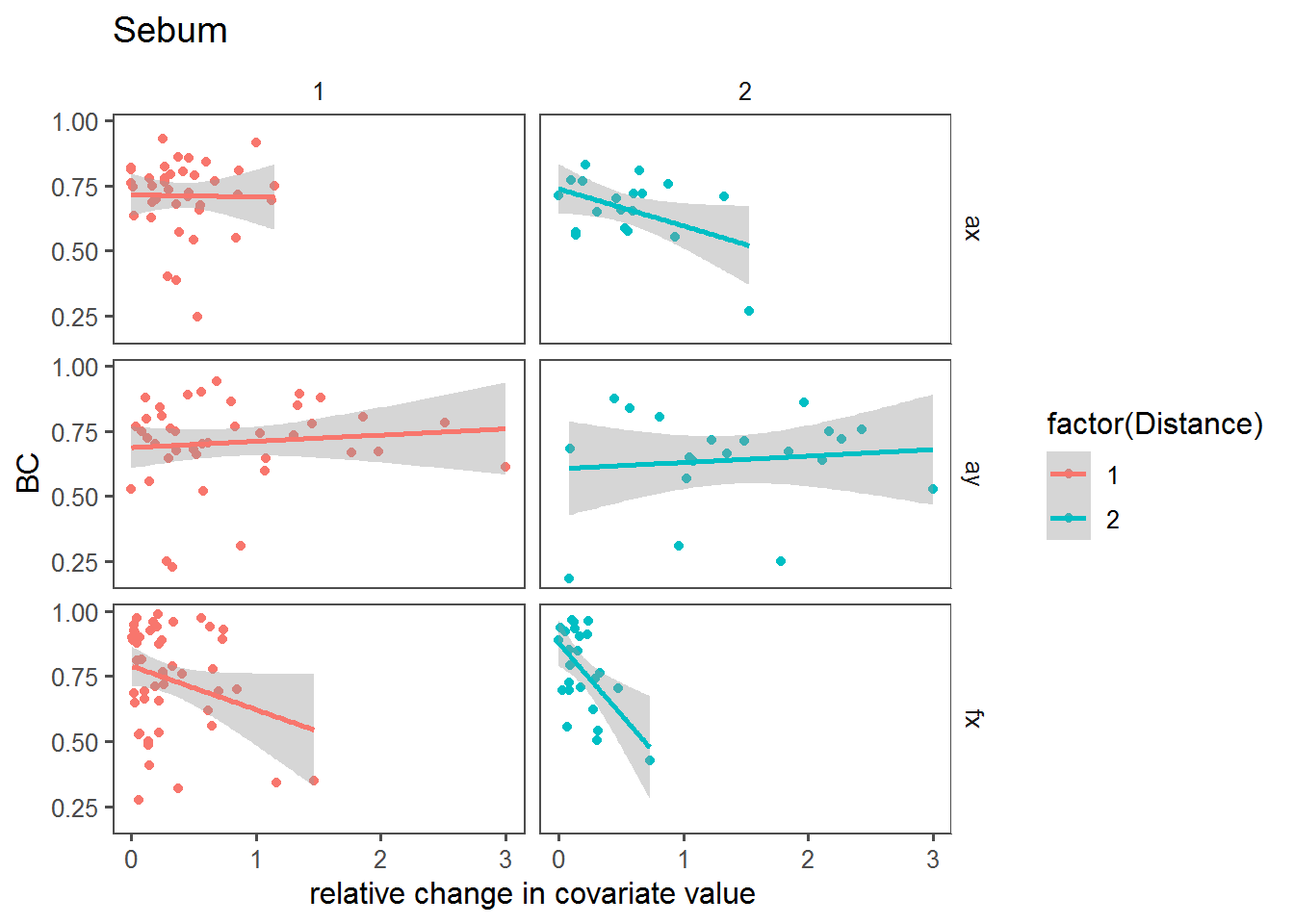

dPlot("Moisture")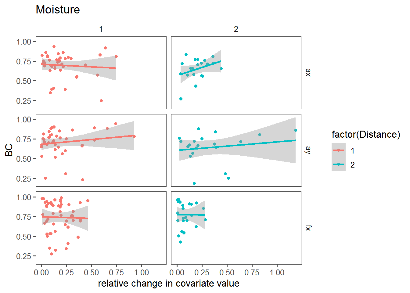

dPlot("Temperature")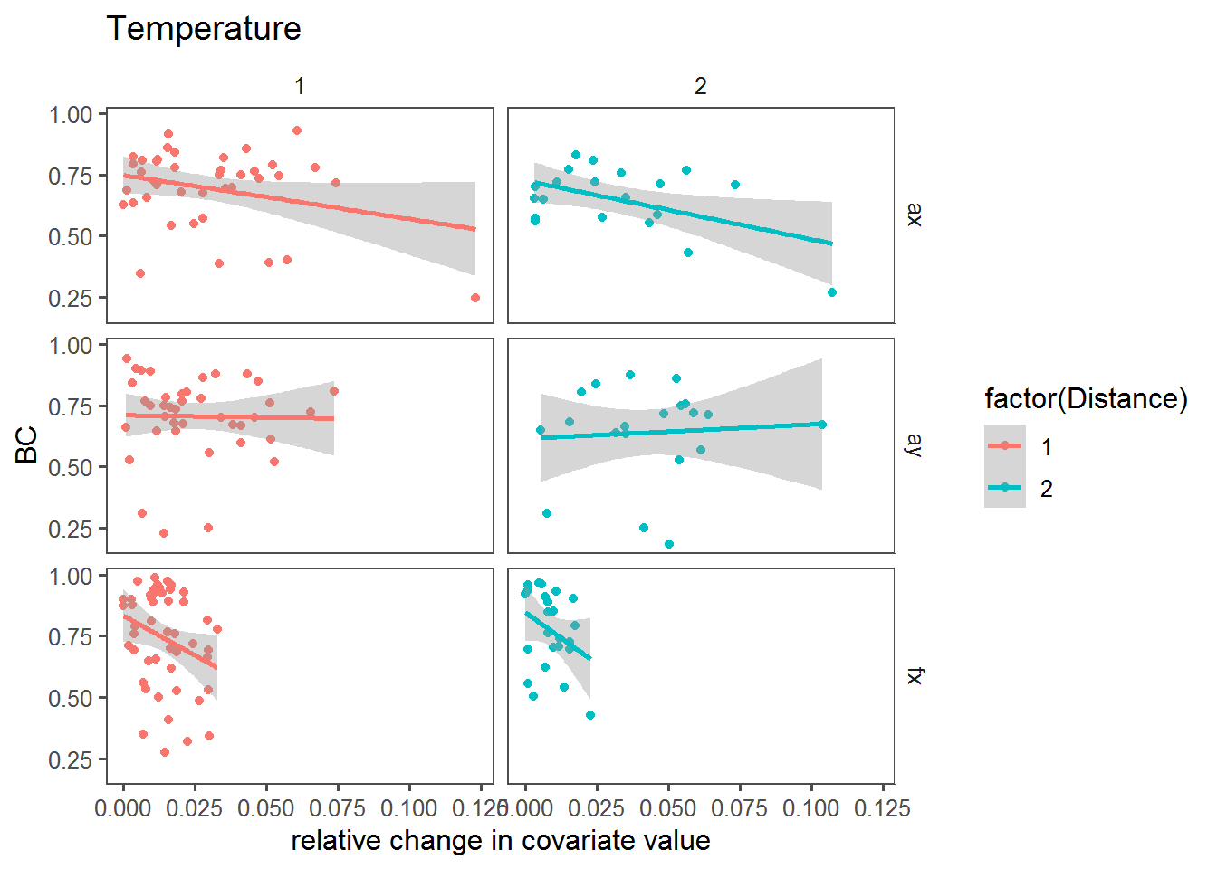

dPlot("pH")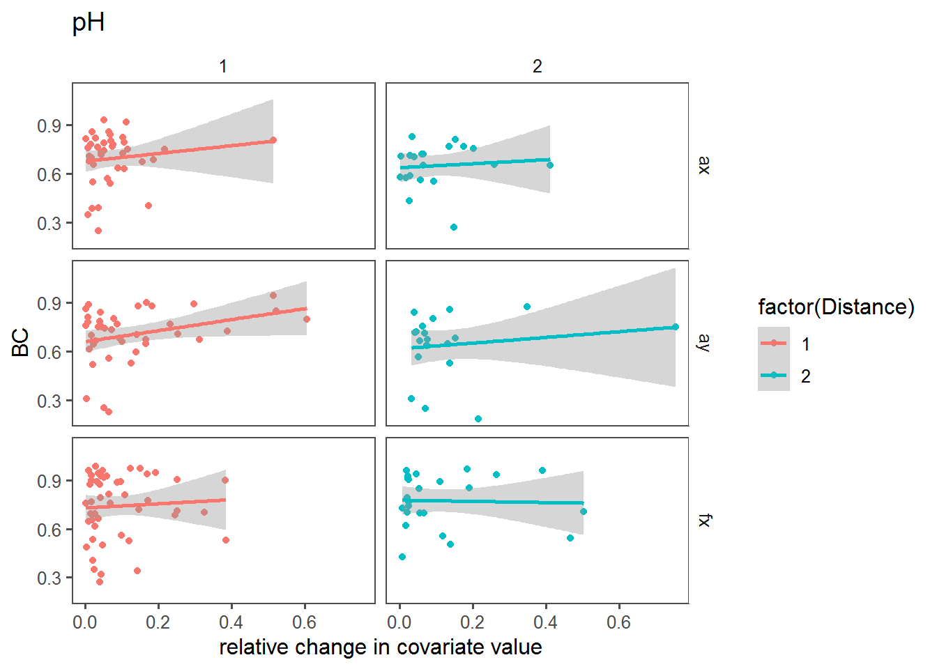

P-values (via a 2-way ANOVA) under 0.1:

df <- subset(T2, Transect == "ax")

RelativeVariableBC.results <- ddply(T2, "Transect", function(df) {
  results <- data.frame(NULL)
  for(cov in covars){
    df2 <- mutate(df, dRel = abs(get(paste0("d",cov))/get(paste0(cov,".mean"))),
                  mono = get(paste0(cov,".mono")))
    mylm <- lm(BC ~ dRel * mono, data = df2)
    
    mytable <- data.frame(cov, beta = mylm$coef[2:4], p.value = anova(mylm)$Pr[1:3])
    row.names(mytable)[2:3] <- c("mono", "interaction")
    mytable$variable <- row.names(mytable)
    results <- rbind(results, mytable)
  }
  return(results)})

RelativeVariableBC.results %>% arrange(p.value) %>% subset(p.value < 0.1)

This suggests

Repeat with only main effects:

df <- subset(T2, Transect == "ax")

RelativeVariableBC.results <- ddply(T2, "Transect", function(df) {
  results <- data.frame(NULL)
  for(cov in covars){
    df2 <- mutate(df, dRel = abs(get(paste0("d",cov))/get(paste0(cov,".mean"))),
                  mono = get(paste0(cov,".mono")))
    mylm <- lm(BC ~ dRel + mono, data = df2)
    
    mytable <- data.frame(cov, beta = mylm$coef[2:3], p.value = anova(mylm)$Pr[1:2])
    mytable$variable <- row.names(mytable)
    results <- rbind(results, mytable)
  }
  return(results)})
RelativeVariableBC.results

subset(RelativeVariableBC.results, p.value < 0.1)

In (almost) no case is the mono main effect significant.

Monotonic change effect

Box plots comparing BC against “mono” (i.e., whether a trend across the transect was monotonous).

bPlot  <- function(cov)
  ggplot(mutate(T2, mono =  get(paste0(cov,".mono"))), 
         aes(x = mono, y = BC, col = factor(Distance))) + facet_grid(Transect~.) + geom_boxplot() + theme_few() + ggtitle(cov) + geom_jitter(alpha=0.2)

bPlot("Sebum")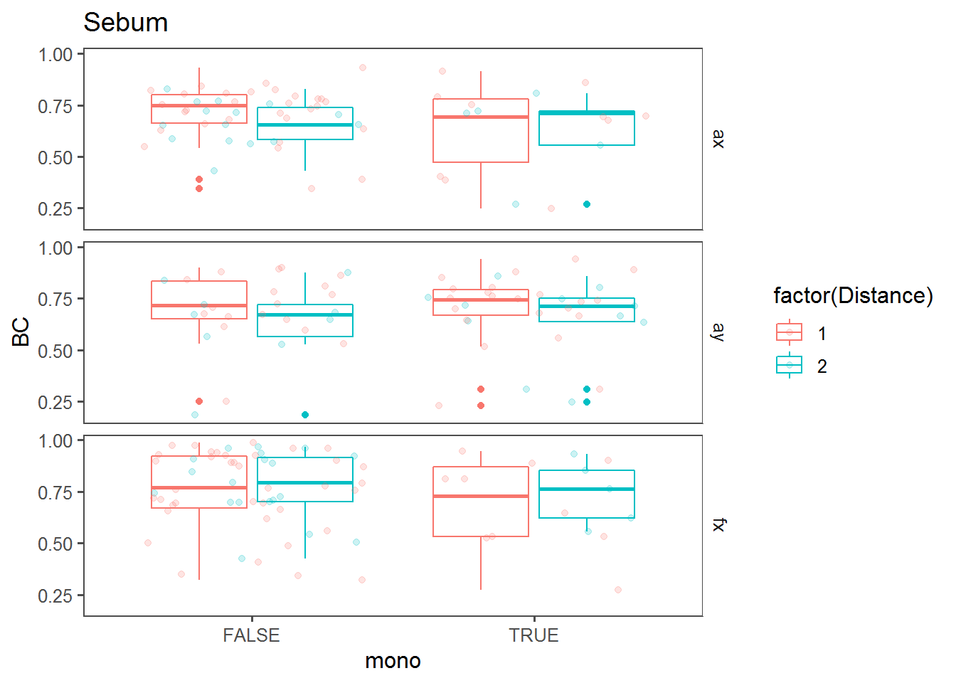

bPlot("Moisture")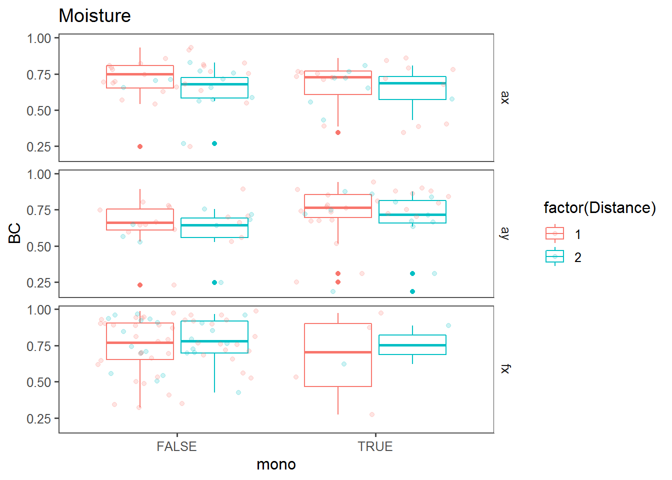

bPlot("Temperature")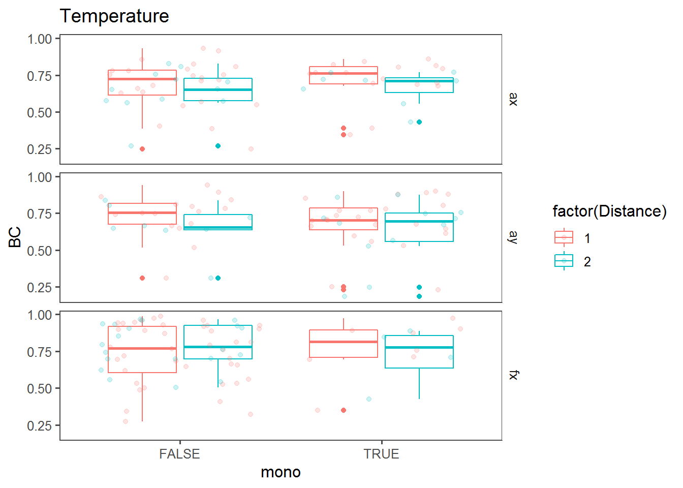

bPlot("pH")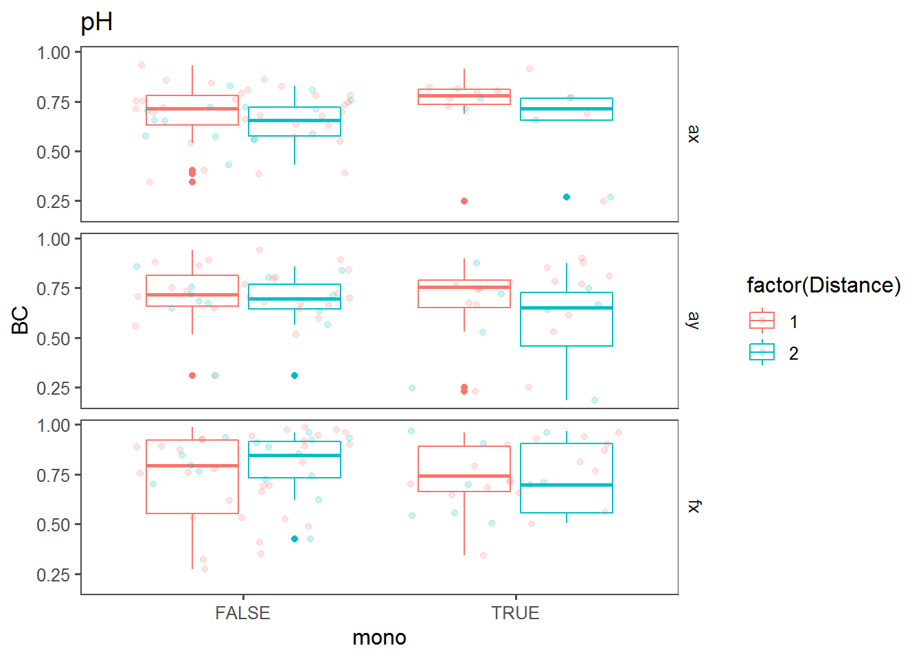

Replicate Sharon’s Chi-squared test

A third way to look at this: Are trends significant against monotonic vs. nonmonotonic probe trends.

T3 <- merge(T.coefs, T2, c("Person","Transect"))
mosaicplot(with(T3, table(Transect, mono = Sebum.mono, signif = beta.pvalue < 0.05)), col = 2:3, main =  "")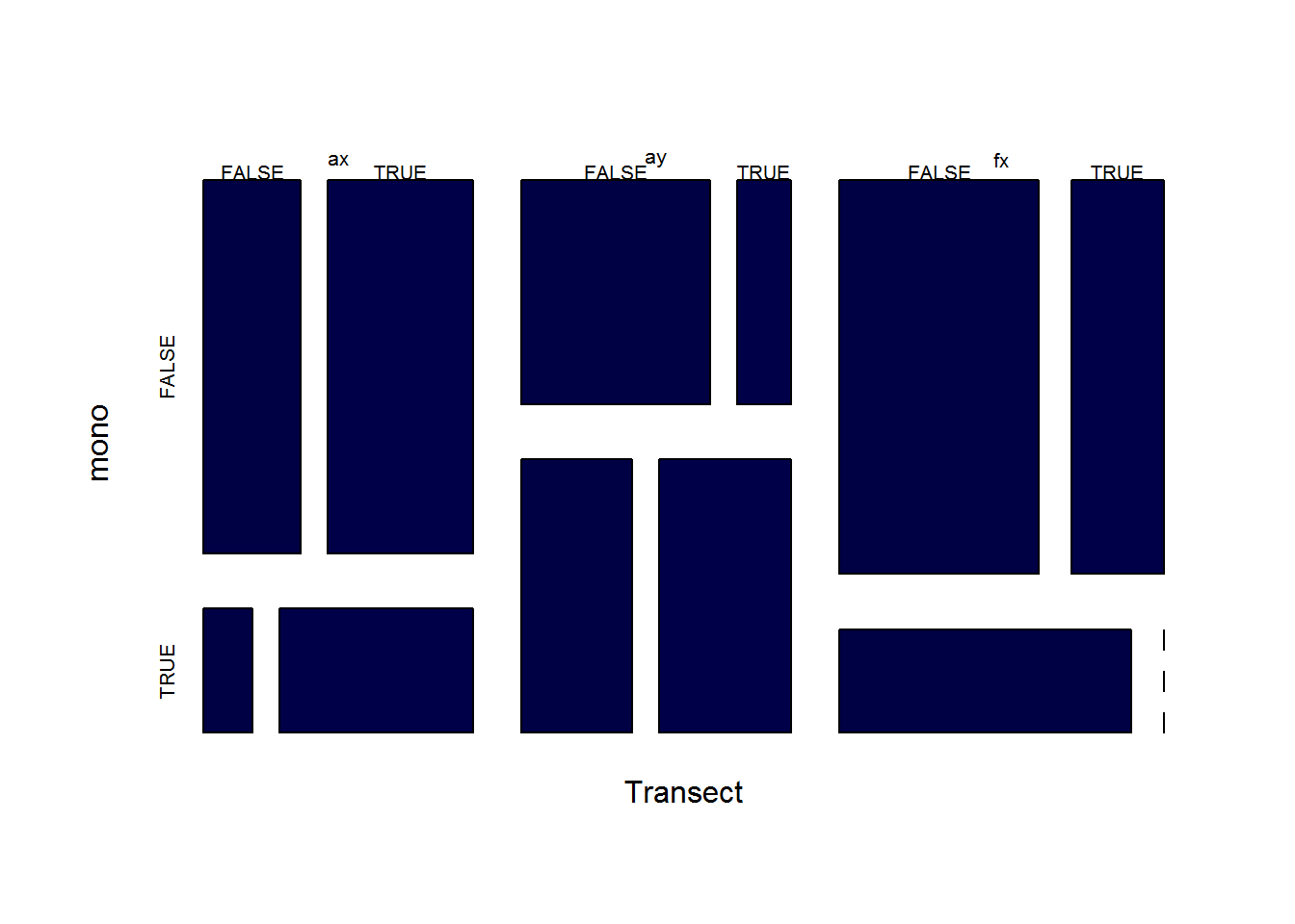

with(subset(T3, Transect == "ax"), table(mono = Sebum.mono, signif = beta.pvalue < 0.05)/3) %T>% print %>% chisq.test

##        signif
## mono    FALSE TRUE
##   FALSE     6    9
##   TRUE      1    4

## 
##  Pearson's Chi-squared test with Yates' continuity correction
## 
## data:  .
## X-squared = 0.07326, df = 1, p-value = 0.7866

with(subset(T3, Transect == "ay"), table(mono = Sebum.mono, signif = beta.pvalue < 0.05)/3) %T>% print %>% chisq.test

##        signif
## mono    FALSE TRUE
##   FALSE     7    2
##   TRUE      5    6

## 
##  Pearson's Chi-squared test with Yates' continuity correction
## 
## data:  .
## X-squared = 1.0185, df = 1, p-value = 0.3129

with(subset(T3, Transect == "fx"), table(mono = Sebum.mono, signif = beta.pvalue < 0.05)/3) %T>% print %>%  chisq.test

##        signif
## mono    FALSE TRUE
##   FALSE    13    6
##   TRUE      5    0

## 
##  Pearson's Chi-squared test with Yates' continuity correction
## 
## data:  .
## X-squared = 0.75789, df = 1, p-value = 0.384