Data loading and processing
The following external package is the only one needed for the code below to work:
require(magrittr)Experimental set-up
There are face and arm transects, which are arranged spatially something like this, though I’m not sure about the numbering (note: the figure below is made in R - click on “show code” to reveal the code):
par(mfrow = c(1,2))
x.X <- -6:6
y.X <- rep(0,13)
x.Y <- rep(0,5)
y.Y <- 0:-4
par(bty="n")
plot(x.X, y.X, pch = 19, type = "o", asp = 1, ylim = c(-5,1), axes=FALSE, xlab="", ylab="", main = "Face Transects")
lines(x.Y, y.Y, typ="o", col=2, pch = 19)
text(x.X, y.X, 1:length(x.X), pos= 3)
text(x.Y, y.Y, pos= 4, col=2)
legend("bottomright", legend = c("Face X", "Face Y"), pch = 19, col=1:2, lty = 1, bty="n")

x.X <- -6:6
y.X <- rep(0,13)
x.Y <- c(-6:0, rep(0,2))
y.Y <- c(rep(-2,7), -1:0)
par(bty="n")
plot(x.X, y.X, pch = 19, type = "o", asp = 1, ylim = c(-2,0.5), axes=FALSE, xlab="", ylab="", main = "Arm Transects")
lines(x.Y, y.Y, typ="o", col=2, pch = 19)
text(x.X, y.X, 1:length(x.X), pos= 3)
text(x.Y[1:6], y.Y[1:6], 9:4, pos= 3, col=2)
text(x.Y[7:9], y.Y[7:9], 3:1, pos= 4, col=2)
legend("bottomright", legend = c("Arm X", "Arm Y"), pch = 19, col=1:2, lty = 1, bty="n")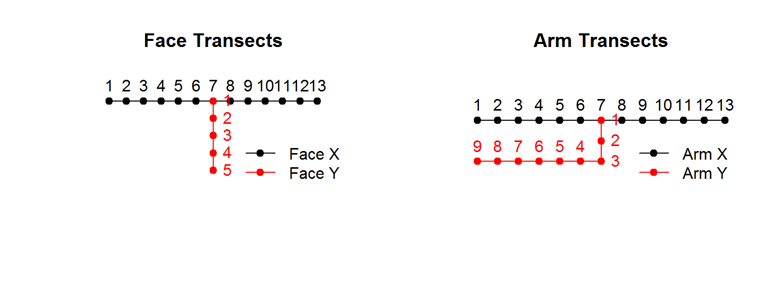
Though the data that we have available actually does not have Face Y nor anything related to depth within skin.
Raw Data
The raw data are stored as site and individual specific files , i.e. the arm X transect files are:
list.files("../data/ax")## [1] "1_ax.csv" "10_ax.csv" "12_ax.csv" "13_ax.csv" "18_ax.csv"
## [6] "19_ax.csv" "20_ax.csv" "23_ax.csv" "24_ax.csv" "25_ax.csv"
## [11] "26_ax.csv" "3_ax.csv" "4_ax.csv" "40_ax.csv" "41_ax.csv"
## [16] "42_ax.csv" "5_ax.csv" "6_ax.csv" "7_ax.csv" "8_ax.csv"
## [21] "9_ax.csv"Where each file represents one individual. This is not a necessary or convenient way to organize the data - so the main goal of the following steps will be to concatenate all of the data into a single file.
Here we load an example raw dataset:
ax4 <- read.csv("../data/ax/4_ax.csv")
ax4 <- cbind(rid = 1:nrow(ax4), ax4)
ax4
Each row is identified by the individual ID, the Transect, the Location (1:12).
The main response variable is Relative_Abundance of the specific Taxon, of which there are 349. Finally, for three of the locations (sites 1, 6 and 12) there are measurements of various skin traits: Sebum, Moisture, Temperature, pH, TEWL, Erythma, Melanin. Obviously, there is a lot of repetition - only 3 measurements per skin property. Here is a table of the unique values:
skintraits <- names(ax4)[7:ncol(ax4)]
ax4[,c("Location",skintraits)] %>% subset(!is.na(Sebum)) %>% unique
Note that the location numberings are different on the different transects. Arm-Y has 7 locations, with measurements on 1, 3 and 7:
ay4 <- read.csv("../data/ay/4_ay.csv")
with(ay4, table(Location))
## Location
## 1 2 3 4 5 6 7
## 349 349 349 349 349 349 349unique(ay4[,c("Location",skintraits)] %>% subset(!is.na(Sebum)))Face X has 7 locations at 1, 3, 7:
fx4 <- read.csv("../data/fx/4_fx.csv")
with(fx4, table(Location))
## Location
## 1 2 3 5 6 7
## 349 349 349 349 349 349unique(fx4[,c("Location",skintraits)] %>% subset(!is.na(Sebum)))Data processing
If the data are, indeed, structured in this way - by individual and by transect, in transect specific folders - then the first thing to do is to combine all of the data into a single data frame so that there is only one data file to keep track of. The following code performs this task:
ax.dir <- "../data/ax/"
ay.dir <- "../data/ay/"
fx.dir <- "../data/fx/"

ax.files <- list.files(ax.dir)
ay.files <- list.files(ay.dir)
fx.files <- list.files(fx.dir)

AX <- data.frame()
for(ax in ax.files) AX <- rbind(AX, read.csv(paste0(ax.dir, ax)))
AY <- data.frame()
for(ay in ay.files) AY <- rbind(AY, read.csv(paste0(ay.dir, ay)))
FX <- data.frame()
for(fx in fx.files) FX <- rbind(FX, read.csv(paste0(fx.dir, fx)))

SMBT <- rbind(data.frame(transect = "ax", AX),
                             data.frame(transect = "ay", AY),
                             data.frame(transect = "fx", FX))
This is a single object - called SMBT for Skin Microbiome Transects, of not inordinate size, but that contains all the data:
dim(SMBT)## [1] 177204 13It should be saved as a text file (e.g. .csv) and/or as an R native data file:
save(SMBT, file = "../data/SMBT.rda")
write.csv(SMBT, file = "../data/SMBT.csv")