Diversity Index
Goals
Here, we replicate much of the analysis from the Species Richness Analysis but, rather than species richness, computing the Simpson index of diversity: \[\lambda = 1-\sum_{i=1}^R p_i^2\] where \(R\) is the richness (number of taxa) and \(p_i\) is the proportional abundance. This index varies from an extreme limit of 0 if a single taxon dominates to 1 (for uniform diversity of infinite number of taxa).
Simpson’s index function
Load the data
load("../data/SMBT.rda")Computing the index is simple:
SI <- function(p) 1 - sum(p^2)Unlike species richness, however, this measure only makes sense at a single location.
SI.df <- ddply(SMBT, c("Transect","Person","Location"), summarize,
               SI = SI(Relative_Abundance))
head(SI.df)
Some boxplots:
require(ggplot2)
require(magrittr)

ggplot(SI.df %>% arrange(SI) %>% mutate(Person = factor(Person, levels = unique(Person))),
       aes(Person, SI)) + geom_boxplot() + facet_wrap(.~Transect) + ylab("Simpson's Index of Diversity")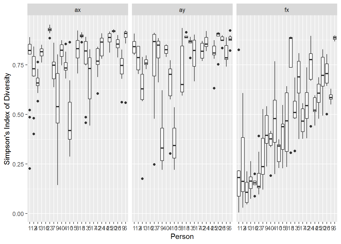
And a mixed effects model of Simpson’s diversity, with Location nested in Person. Note that because of the nesting, this model can take a while to fit:
require(nlme)
SI.lme <- lme(SI ~ Transect - 1, random = ~ (Transect-1)|Person/Location,
                  data = SI.df)
Differences across transects are stark, with a considerably higher SI on the arm (0.77 and 0.75 for X and Y [though within a standard error), and much lower on the face (0.46):
summary(SI.lme)$tTable## Value Std.Error DF t-value p-value
## Transectax 0.7700281 0.02481385 289 31.03219 5.293335e-94
## Transectay 0.7509939 0.03217303 289 23.34234 1.837143e-68
## Transectfx 0.4589086 0.04235588 289 10.83459 3.506714e-23This inter-individal and intra-individual variability is, however, also quite high:
VarCorr(SI.lme)## Variance StdDev Corr
## Person = pdLogChol((Transect - 1))
## Transectax 0.012358008 0.11116658 Trnsctx Trnscty
## Transectay 0.020951018 0.14474466 0.855
## Transectfx 0.042182256 0.20538319 0.414 0.504
## Location = pdLogChol((Transect - 1))
## Transectax 0.008910249 0.09439412 Trnsctx Trnscty
## Transectay 0.009601950 0.09798954 -0.057
## Transectfx 0.016280454 0.12759488 0.158 0.094
## Residual 0.001465691 0.03828434i.e., the standard deviation across people ranges from 0.1 (for arm) to 0.2 (for face), with a relatively correlation across those factors (e.g. 0.8 for Arm X and Arm Y). Within people that standard deviation is consistently approximately 0.1.
SI against covariates
We repeat the analysis from the previous section to see if any of the environmental covariates have any predictive power for explaining the diversity.
covariates <-  c("Moisture", "Temperature", "pH", "Sebum")
covars.df <- SMBT[,c("Transect", "Person", "Location", covariates)] %>% na.omit %>% unique
SI.covars.df <- merge(covars.df, SI.df)
Pairs plot
require(GGally); require(ggthemes)
ggpairs(SI.covars.df, aes(col = Transect), columns = c("SI", covariates)) + theme_few()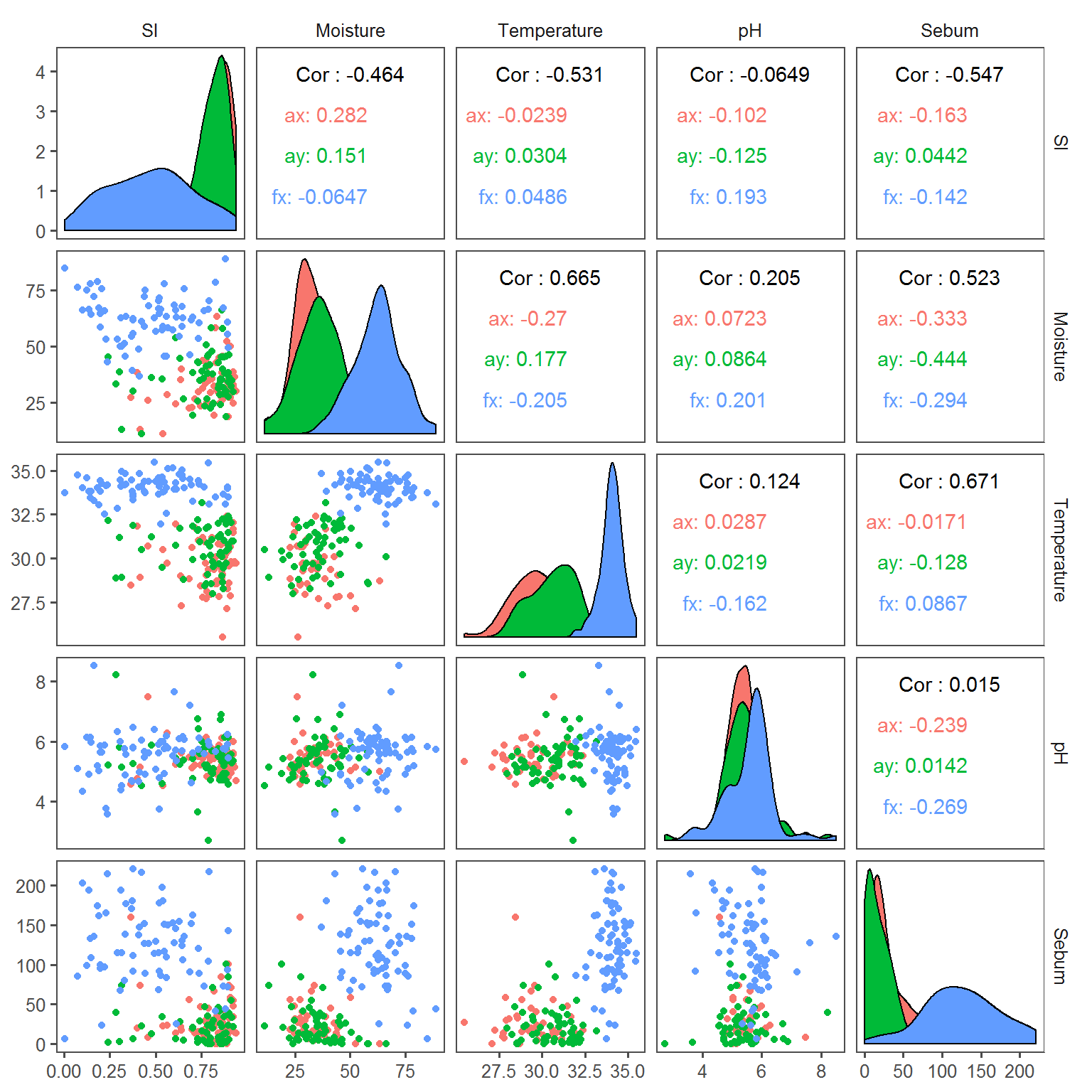
Most transect-specific correlations appear rather weak, but the high level of variability among and within individuals may swamp some patterns.
Mixed-effects models
We’ll need the following packages:
require(nlme)
require(MuMIn)
f <- SI ~ (Sebum + Temperature + pH + Moisture)^2
Click on tabs to see tables and plots of model selection
AX dredge
ax.lme <- lme(f, random = ~1|Person/Location, data = SI.covars.df,
    subset = Transect == "ax" & !is.na(Sebum), method = "ML")
(ax.dredge <- dredge(ax.lme))
plot(ax.dredge)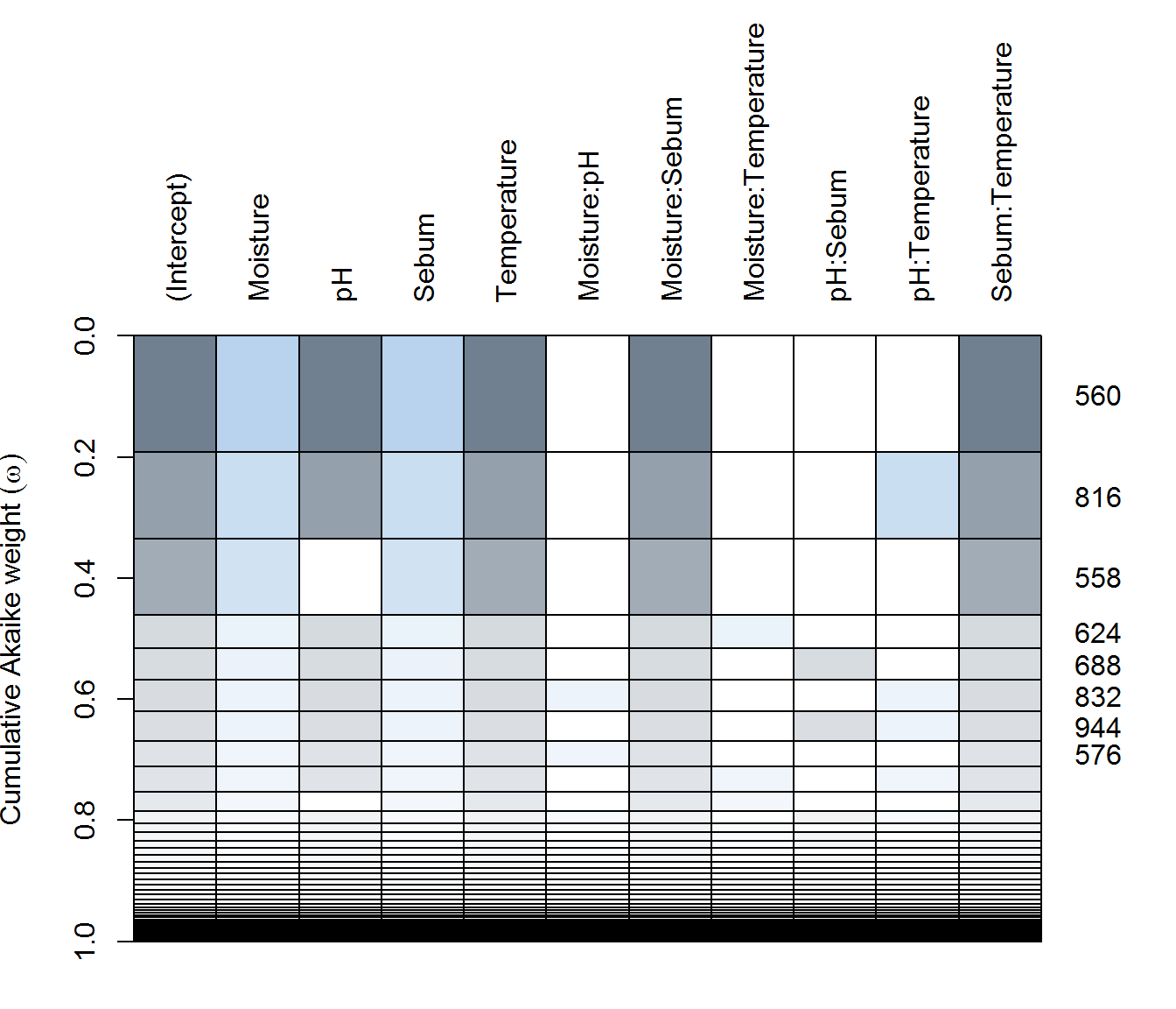
AY dredge
ay.lme <- lme(f, random = ~1|Person/Location, data = SI.covars.df,
    subset = Transect == "ay" & !is.na(Sebum), method = "ML")
(ay.dredge <- dredge(ay.lme))
plot(ay.dredge)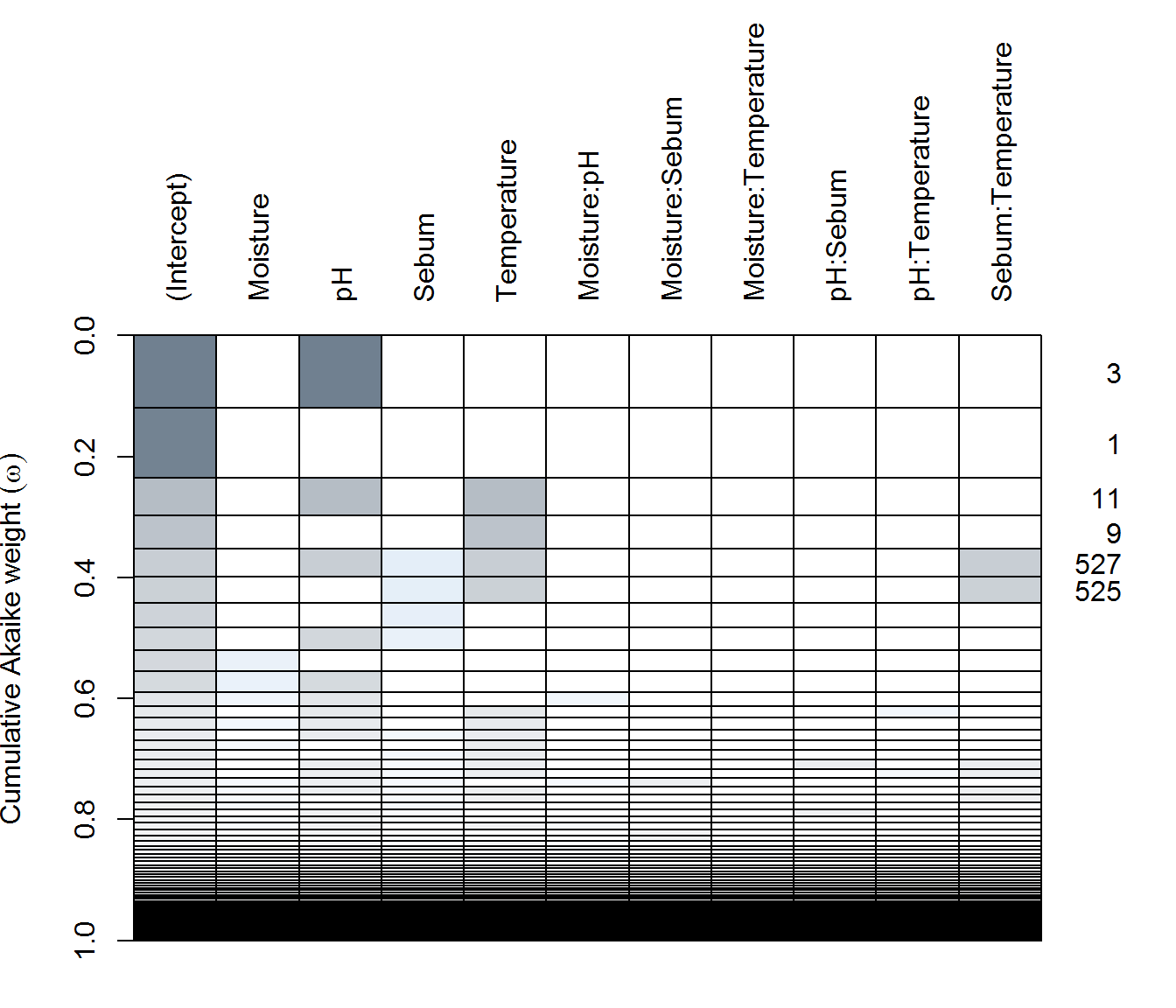
FX dredge
fx.lme <- lme(f, random = ~1|Person/Location, data = SI.covars.df,
    subset = Transect == "fx" & !is.na(Sebum), method = "ML")
(fx.dredge <- dredge(fx.lme))
plot(fx.dredge)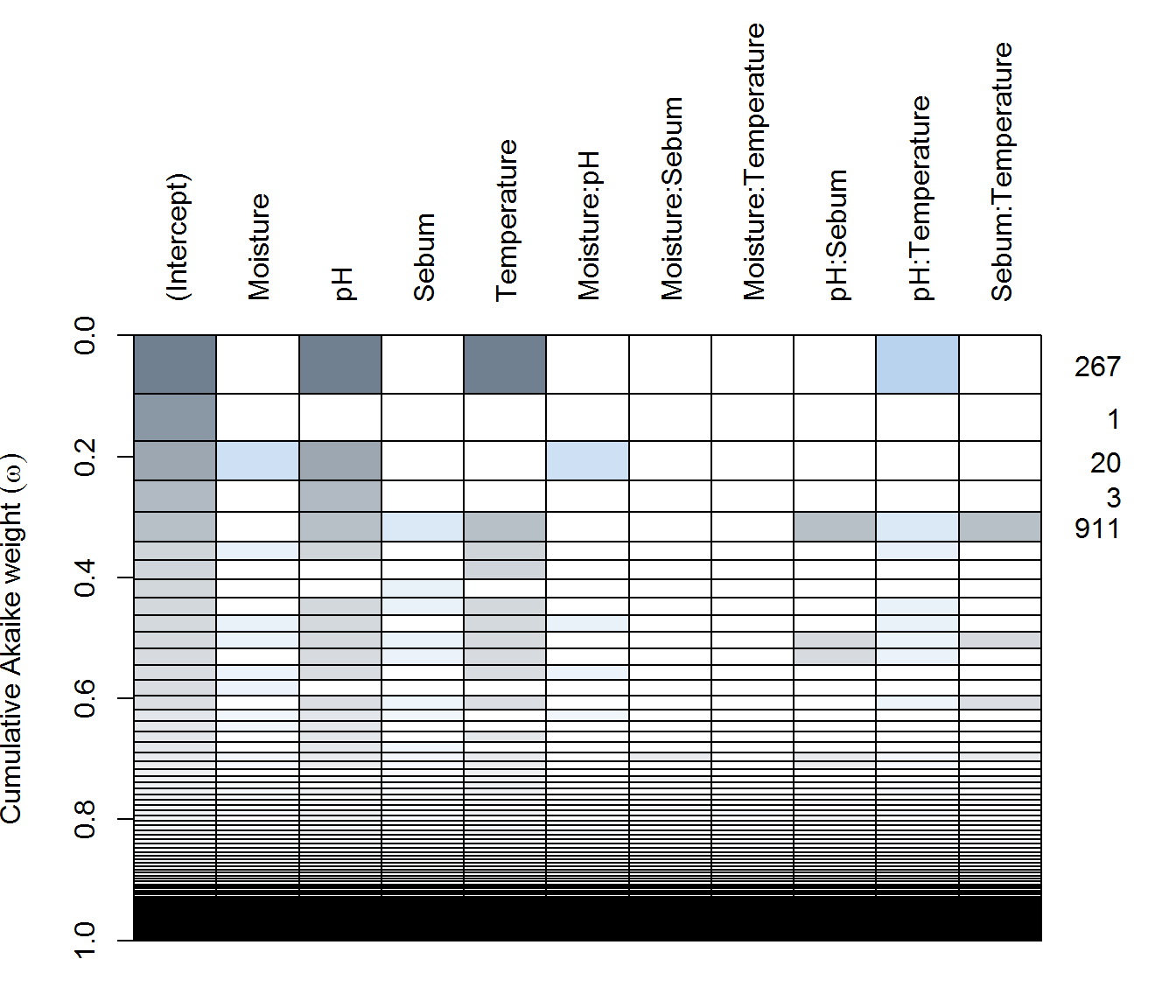
There are some differences, with Arm-X showing the strongest explanatory power by various covariates, but weak explanatory power for Arm-Y and Face.
Parameter estimates
Coefficients for “best” (or near best) models:
SI.covars.scaled <- mutate(SI.covars.df, pH = scale(pH), Moisture = scale (Moisture), Sebum = scale(Sebum), Temperature = scale(Temperature))

fitted.models <- list(
  AX = lme(SI ~ Moisture + pH + Sebum*(Moisture + Temperature), random = ~1|Person/Location,
           data = SI.covars.scaled, subset = Transect == "ax"),
  AY = lme(SI ~ pH + Temperature, random = ~1|Person/Location,
           data = SI.covars.scaled, subset = Transect == "ay"),
  FX =  lme(SI ~ pH * Temperature, random = ~1|Person/Location,
            data = SI.covars.scaled, subset = Transect == "fx"))
require(broom); require(ggthemes)
results <- ldply(fitted.models, tidy, effects = "fixed")
ggplot(results %>% subset(term != "(Intercept)") %>%
         mutate(p.value = cut(p.value, c(0, 0.05, 0.1, 1))),
       aes(estimate, term, col = p.value)) +
  geom_vline(xintercept = 0, col = "darkgrey") +
  geom_errorbarh(aes(xmin = estimate - 2*std.error, xmax = estimate + 2*std.error), lwd = 1, height = 0.3) + facet_wrap(.~.id)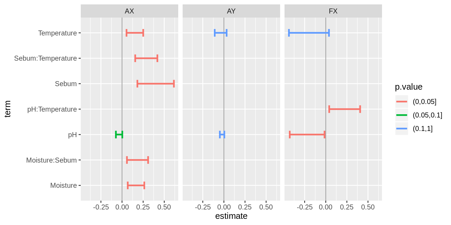
I guess a take-away is that acidic skin tends to have lower diversity.