Appendix AA. Computer simulation of signals and instruments.

Throughout this book, I have often used computer simulations to test, demonstrate, and determine the range of applicability and the accuracy of various signal processing techniques. The aim is to generate realistic computer-simulated signal by adding together three components:

(a) known signal component, such as one or more peaks, pulses, or sigmoidal steps,
(b) a baseline, which may be fixed, variable, flat, sloped, curved or stepped, and
(c) random noise, which may have various frequency distributions (colors) and amplitude dependencies. 


Such simulations can be done either in Matlab/Octave, using the built-in and downloadable functions for various peak shapes 
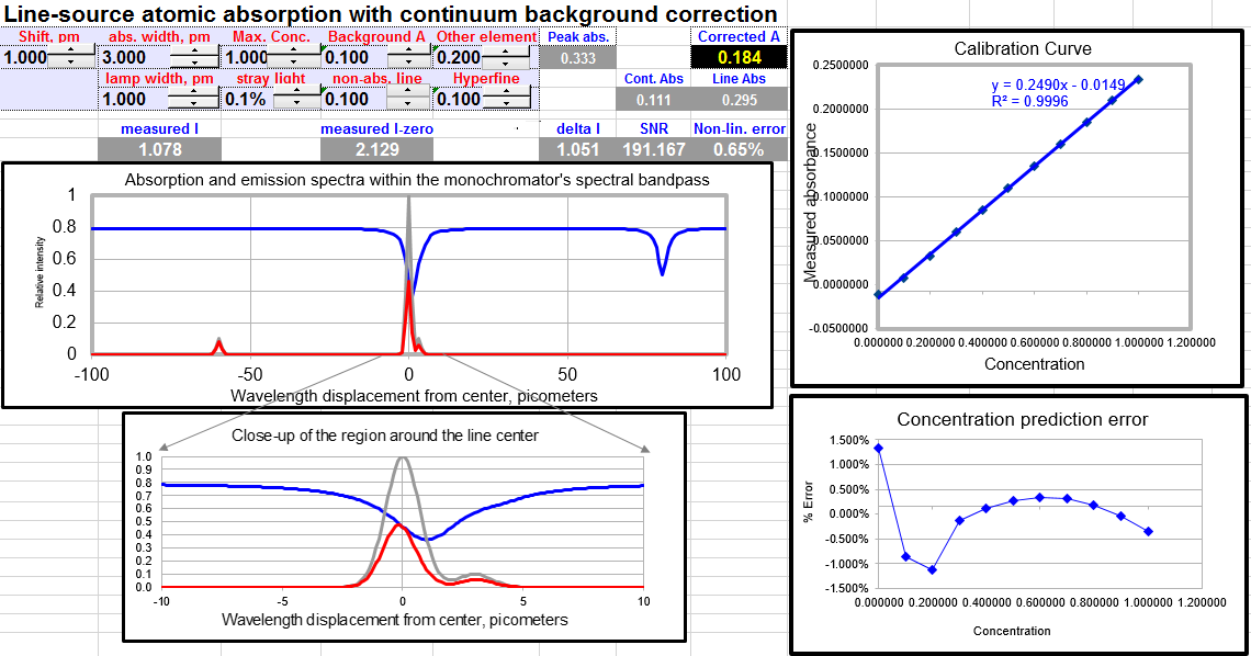
and types of random noise, or in spreadsheets, which can also be used to create attractive and intuitive user interfaces; some spreadsheet examples include SimulatedSignal6Gaussian.xlsx, PeakSharpeningDemo.xlsx, PeakDetectionDemo2.xls, TransmissionFittingDemoGaussian.xls, BeersLawCurveFit2.xls, and RegressionDemo.xls (above).

It's possible to make any aspect of a computer generated signal randomly variable from measurement to measurement, with the aim of making  the simulation as close as possible to the real signal behavior that you may have to measure. For example, in section E, "The Battle Rounds: a comparison of methods", the signal to be measured is a Gaussian peak located near the center of the recorded signal, with a fixed shape and width. The baseline, on the other hand, is highly variable, both in amplitude and in shape, and there is also added white noise. In another simulation, "Why measure peak area rather than peak height?", the signal peak itself is subject to a variable broadening process that causes the measured peak to be shorter and wider but which has no effect of the total area. In the section "Measuring a buried peak", the signal is a small "child" peak that is buried under the tail of a much stronger "parent" peak. In all these cases, the true underlying signal is known to the software, so that, after the software measures the simulated observed signal with all its baseline and noise variability, it can calculate the error of measurement, allowing you to compare different methods ’
or to optimize the method's variables to obtain the best accuracy.

Modeling instrument systems. In some cases it may be possible to simulate important aspects of entire measurement instrument systems for instructional and training purposes. Several examples are shown in https://terpconnect.umd.edu/~toh/models/. This is most useful if both the signal magnitude and the noise can be predicted from first principles. For example, in optical spectroscopy, the principles of physics and of geometrical optics can be used to predict the intensity of an incandescent light source, the transmission of a monochromator, and the signal generated by a photomultiplier, including the photon noise.


When these are combined, it's possible to simulate the fundamental aspects of such instruments as a scanning fluorescence spectrometer (above) or an atomic absorption instrument (below),


to predict the analytical calibration curves of absorption spectroscopy, to compare the theoretical signal-to-noise ratios of absorption and fluorescence measurement, and to predict the detection limits of atomic emission measurement of various elements, and the effect of slit width on signal-to-noise ratio in absorption spectroscopy (below).


You can also simulate the operation of a lock-in amplifier, a wavelength modulation spectroscopy system, and even basic analog electronic and operational amplifier circuits. Note that these are not simulations of particular commercial instruments, nor are they training tools for instrument operators. Rather, they are interactively manipulated mathematical models that describe various parts of or aspects of each system, for the purpose of illuminating hidden aspects of the instrument's internal operation.


This page is part of "A Pragmatic Introduction to Signal Processing", created and maintained by Prof. Tom O'Haver , Department of Chemistry and Biochemistry, The University of Maryland at College Park. Comments, suggestions and questions should be directed to Prof. O'Haver at toh@umd.edu. Updated July, 2022.