SegmentedSmooth.m, illustrated on the right, is a segmented
variant of fastsmooth.m,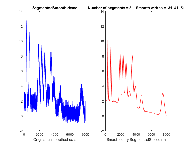 which can be useful if the widths of the peaks or the
noise level varies substantially across the signal. The
syntax is that same as fastsmooth.m, except that the
second input argument "smoothwidths" can be a vector: SmoothY =
SegmentedSmooth (Y, smoothwidths,type,ends). The function divides Y into
a number of equal-length regions defined by the length
of the vector 'smoothwidths', then smooths each region
with a smooth of type 'type' and width defined by the
elements of vector 'smoothwidths'. In the simple example
in the figure on the right, smoothwidths=[31
52
91], which divides up the signal
into three regions and smooths the first region with
smoothwidth 31, the second with 51, and the last with
91. Any number and sequence of
smooth widths can be used. If the peak widths increase
or decrease regularly across the signal, you can
calculate the smoothwidths vector by giving only the
number of segments ("NumSegments") , the first value,
"startw", and the last value, "endw", like so:
which can be useful if the widths of the peaks or the
noise level varies substantially across the signal. The
syntax is that same as fastsmooth.m, except that the
second input argument "smoothwidths" can be a vector: SmoothY =
SegmentedSmooth (Y, smoothwidths,type,ends). The function divides Y into
a number of equal-length regions defined by the length
of the vector 'smoothwidths', then smooths each region
with a smooth of type 'type' and width defined by the
elements of vector 'smoothwidths'. In the simple example
in the figure on the right, smoothwidths=[31
52
91], which divides up the signal
into three regions and smooths the first region with
smoothwidth 31, the second with 51, and the last with
91. Any number and sequence of
smooth widths can be used. If the peak widths increase
or decrease regularly across the signal, you can
calculate the smoothwidths vector by giving only the
number of segments ("NumSegments") , the first value,
"startw", and the last value, "endw", like so:
wstep=(endw-startw)/NumSegments;
smoothwidths=startw:wstep:endw;
Type "help
SegmentedSmooth" for other examples examples. DemoSegmentedSmooth.m
demonstrates the operation
with different signals consisting of noisy
variable-width peaks that get progressively wider, like
the figure on the right. FindpeaksSL.m is the same thing
for Lorentzian peaks.
SegmentedSmoothTemplate.xlsx is
a segmented multiple-width data
smoothing spreadsheet template, functionally similar to
SegmentedSmooth.m. In this version there are 20 segments. SegmentedSmoothExample.xlsx is
an example with data (graphic). A related
spreadsheet GradientSmoothTemplate.xlsx (graphic) performs a linearly increasing (or decreasing) smooth
width across the entire signal, given only the start and end
values, automatically generating as many segments are are
necessary. Of course, as is usual with spreadsheets, you'll have
to modify these templates for your particular number of data
points, usually by inserting rows somewhere in the middle and
then drag-copying down from above the insert, plus you may have
to change the x-axis range of the graph. (In contrast, the
Matlab/Octave functions do that automatically).
Segmented Fourier filter. SegmentedFouFilter.m is a segmented
version of FouFilter.m, which applies
different center frequencies and widths to different segments of
the signal. The syntax is the same as FouFilter.m except that
the two input arguments 'centerFrequency' and 'filterWidth' must
be vectors with the values of centerFrequency of filterWidth for
each segment. The signal is divided equally into a number of
segments determined by the length of centerFrequency and
filterWidth, which must be equal. Type 'help SegmentedFouFilter'
for help and examples.
findpeaksSG.m is a variant of the findpeaksG function, with
the same syntax, except that the four peak detection
parameters can be vectors, dividing up the signal into regions that are
optimized for peaks of different widths. Any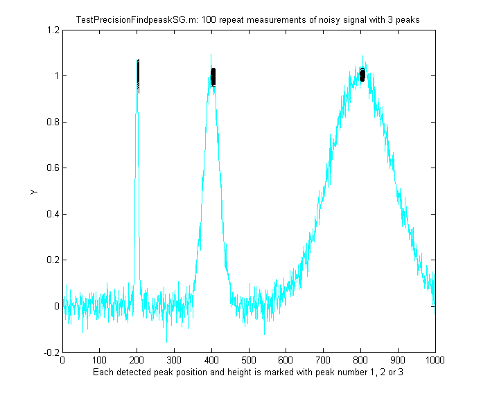 number of segments can be declared, based on the
lengths of the SlopeThreshold input argument. (Note: you
need only enter vectors for those parameters that you
want to vary between segments; to allow any of the other
peak detection parameters to remain unchanged across all
segments, simply enter a single scalar value for that
parameter; only the SlopeThreshold must be a vector). In
the example shown on the left,
the script TestPrecisionFindpeaksSG.m creates a noisy signal with
three peaks of widely different widths, measures the
peak positions, heights and widths of each peak using
findpeaksSG, and prints out the percent relative
standard deviations of parameters of the three peaks in
100 measurements with independent random noise. With
3-segment peak detection parameters, findpeaksSG
reliably detects and accurately measures all three
peaks. In contrast, findpeaksG, tuned to the middle peak
(using line 26 instead of line 25), measures the first
and last peaks poorly. You can also see that the
precision of peak parameter measurements gets
progressively better (smaller relative standard
deviation) the larger the peak widths, simply because
there are more data points in those peaks. (You can
change any of the variables in lines 10-18).
number of segments can be declared, based on the
lengths of the SlopeThreshold input argument. (Note: you
need only enter vectors for those parameters that you
want to vary between segments; to allow any of the other
peak detection parameters to remain unchanged across all
segments, simply enter a single scalar value for that
parameter; only the SlopeThreshold must be a vector). In
the example shown on the left,
the script TestPrecisionFindpeaksSG.m creates a noisy signal with
three peaks of widely different widths, measures the
peak positions, heights and widths of each peak using
findpeaksSG, and prints out the percent relative
standard deviations of parameters of the three peaks in
100 measurements with independent random noise. With
3-segment peak detection parameters, findpeaksSG
reliably detects and accurately measures all three
peaks. In contrast, findpeaksG, tuned to the middle peak
(using line 26 instead of line 25), measures the first
and last peaks poorly. You can also see that the
precision of peak parameter measurements gets
progressively better (smaller relative standard
deviation) the larger the peak widths, simply because
there are more data points in those peaks. (You can
change any of the variables in lines 10-18).
findpeaksSb.m is a segmented variant of
the findpeaksb.m function. 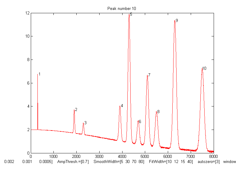 It
has the same syntax as findpeaksSb, except that the
arguments "SlopeThreshold", "AmpThreshold",
"smoothwidth", "peakgroup", "window", "PeakShape",
"extra", "NumTrials", "autozero", and "fixedparameters"
can all be optionally scalars or vectors with one entry for
each segment. This allows the function to handle widely
varying signals with peaks of very different shapes and
widths and backgrounds. In the example on the right, the
Matlab/Octave script DemoFindPeaksSb.m creates a series of Gaussian
peaks whose widths increase by a factor of 25 and that are superimposed in
a curved baseline with random white noise that increases
gradually across the signal. In this example, four segments are used, changing the peak
detection and curve fitting values so that all the peaks
are measured accurately.
It
has the same syntax as findpeaksSb, except that the
arguments "SlopeThreshold", "AmpThreshold",
"smoothwidth", "peakgroup", "window", "PeakShape",
"extra", "NumTrials", "autozero", and "fixedparameters"
can all be optionally scalars or vectors with one entry for
each segment. This allows the function to handle widely
varying signals with peaks of very different shapes and
widths and backgrounds. In the example on the right, the
Matlab/Octave script DemoFindPeaksSb.m creates a series of Gaussian
peaks whose widths increase by a factor of 25 and that are superimposed in
a curved baseline with random white noise that increases
gradually across the signal. In this example, four segments are used, changing the peak
detection and curve fitting values so that all the peaks
are measured accurately.
SlopeThreshold
= [.01 .005 .002 .001];
AmpThreshold = 0.7;
SmoothWidth = [5 15 30 35];
FitWidth = [10 12 15 20];
windowspan = [100 125 150 200];
peakshape = 1;
autozero = 3;
The script also computes
the relative percent error of the measurement of peak
position, height, width, and area for each peak.
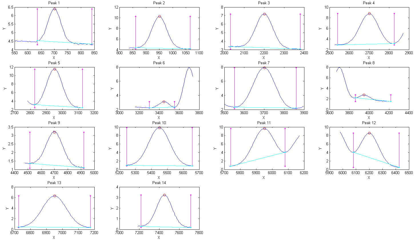 perpendicular drop area
is the total area measured between the two magenta vertical lines
down to zero, and the tangent skim area is the area between the
cyan baseline and the blue peak (which compensates for a flat
baseline). Type "help measurepeaks" and try the examples there or
run testmeasurepeaks.m
(graphic
animation). The related functions autopeaks.m and autopeaksplot.m
are similar, except that the four peak detection parameters can be omitted and the function will calculate estimated initial values.
perpendicular drop area
is the total area measured between the two magenta vertical lines
down to zero, and the tangent skim area is the area between the
cyan baseline and the blue peak (which compensates for a flat
baseline). Type "help measurepeaks" and try the examples there or
run testmeasurepeaks.m
(graphic
animation). The related functions autopeaks.m and autopeaksplot.m
are similar, except that the four peak detection parameters can be omitted and the function will calculate estimated initial values.
The script HeightAndArea.m
tests the accuracy of peak height and area measurement with
signals that have multiple peaks with variable width, noise,
background, and peak overlap. Generally, the values for absolute
peak height and perpendicular drop area are best for peaks that
have no background, even if they are slightly overlapped,
whereas the values for peak-valley difference and for tangential
skim area are better for isolated peaks on a straight or
slightly curved background. Note: this function uses smoothing
(specified by the SmoothWidth input argument) only for peak
detection; it performs its measurements on the raw unsmoothed y
data. If the raw data are noisy, it may be best to smooth the y
data yourself before calling measurepeaks.m, using any smooth
function of your choice.
Other segmented functions. The same segmentation code used in SegmentedSmooth.m
(lines 53-65) can be applied to other functions simply by
editing the first line in the first for/end loop (line 59) to
refer to the function that you want to apply in a segmented
fashion. For example, segmented peak sharpening can be useful when
a signal has multiple peaks that vary in width, and segmented deconvolution
can be useful when a signal has multiple peaks that vary in
width or tailing vary substantially across the signal: SegExpDeconv(x,y,tc)
deconvolutes y with a vector of exponential functions whose time
constants are specified by the vector tc. SegExpDeconvPlot.m
is the same except that it plots the original and deconvoluted
signals and shows the divisions
between the segments by vertical magenta lines.