Spatial Analysis In R
Elie and Silvia (with thanks to T. Barry, G. Wittemyer, M. Hebblewhite)
July 22, 2017
Background
Animals live and move in structured, heterogeneous space. Most analyses of movement are not limited to describing the properties of displacement, but ask some questions with respect to spatial variables. Spatial data objects in R can be rather complex - broadly, a landscape can be described in terms of vectors, which include polygons (e.g. - boundaries of a projected area), lines (e.g. roads), points (e.g. houses) or in terms of a raster which is just a grid (usually square) where each cell has a particular value, whether discrete (e.g. a land-cover type) or continuous (e.g. an elevation).
There are some packages that are very helpful for working with raster and spatial data. Here’s a listm, in approximate decreasing order of usefulness:
spprovides the classes for spatial data; makes coordinate transformations simplerastergeneral-purpose raster functions; reads raster objects into R (very fast)rgdalreads shape files into Rrgeosa collection of excellent methods for working with spatial objectsspatstatnitty-gritty spatial calculations in compiled C code; model-fittingadehabitatHRtools for home range estimation, such as 95% MCPmaptoolsconversion between spatstat and spatial objectsadehabitatMAfunctions that make it easier to work rastersmapdataa collection of map databases, though you might find higher-resolution maps elsewhere
In this lab, we will:
- Load a shape file of Banff National Park in Canada (obtained from the internet)
- Load raster files of land cover types and elevation from the National Park
- Load movement data of elk and moose from Banff
- Obtain some comparative summaries of habitat use
- Estimate a resource selection function (RSF).
Loading a shape file
From Wikipedia: The shapefile format is a popular geospatial vector data format for geographic information system (GIS) software. It is developed and regulated by Esri as a (mostly) open specification for data interoperability among Esri and other GIS software products. In practice, is is actually several files, all of which have the same name and the following extentions:
.shp— shape format; the feature geometry itself.shx— shape index format; a positional index of the feature geometry to allow seeking forwards and backwards quickly.dbf— attribute format; columnar attributes for each shape, in dBase IV format.prj— projection format; the coordinate system and projection information, a plain text file describing the projection using well-known text format.
(NB: This list is not complete - see the Wikipedia page).
You can download shape files for any protected area on earth from https://www.protectedplanet.net, including Banff National Park in Canada (click link for source of shape file).
We downloaded and renamed this file and placed them in the banff folder here: https://terpconnect.umd.edu/~egurarie/teaching/MovementAtICCB2017/data/ You can download those files (either separately, or the zip file), place them somewhere useful on your computer, and load them with the readOGR command.
require(rgdal)
banff <- readOGR("./_data/banff")
## OGR data source with driver: ESRI Shapefile
## Source: "./_data/banff", layer: "BanffNationalPark"
## with 1 features
## It has 28 fields
## Integer64 fields read as strings: STATUS_YR METADATAIDplot(banff, main = "Banff N.P.", axes=TRUE, col="green")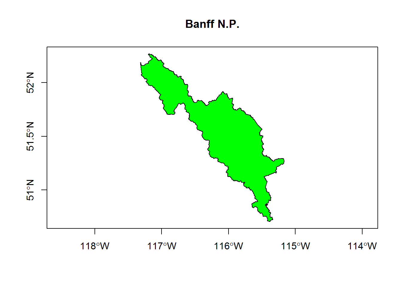
Note, banff is an exotic object called a SpatialPolygonsDataFrame, which contains a lot of important spatial information but (in this case) just one set of coordinates for a single polygon. Important features of this object include:
- The polygon information (only one row!)
banff@data## WDPAID WDPA_PID PA_DEF NAME
## 0 615 615 1 Banff National Park of Canada
## ORIG_NAME DESIG
## 0 Banff National Park of Canada National Park of Canada
## DESIG_ENG DESIG_TYPE IUCN_CAT INT_CRIT MARINE
## 0 National Park of Canada National II Not Applicable 0
## REP_M_AREA GIS_M_AREA REP_AREA GIS_AREA NO_TAKE NO_TK_AREA
## 0 0 0 6641 6846.905 Not Applicable 0
## STATUS STATUS_YR GOV_TYPE OWN_TYPE
## 0 Designated 1885 Federal or national ministry or agency State
## MANG_AUTH
## 0 Government of Canada, Parks Canada Agency
## MANG_PLAN VERIF METADATAID SUB_LOC
## 0 http://www.pc.gc.ca/index_e.asp State Verified 1868 CA-AB
## PARENT_ISO ISO3
## 0 CAN CAN- the projection
banff@proj4string## CRS arguments:
## +proj=longlat +datum=WGS84 +no_defs +ellps=WGS84 +towgs84=0,0,0- the boundary box
bbox(banff)## min max
## x -117.31708 -115.16491
## y 50.70506 52.27036- the coordinates of the one polygon (very tedious!)
banff.ll <- banff@polygons[[1]]@Polygons[[1]]@coordsA quick ggmap of the park boundaries:
require(ggmap)
require(scales)
mymap <- get_map(bbox(banff), maptype= "terrain", zoom = 8)
ggmap(mymap) + geom_polygon(data = data.frame(banff.ll), aes(x = X1, y = X2), fill = alpha("pink", .2), col="darkred")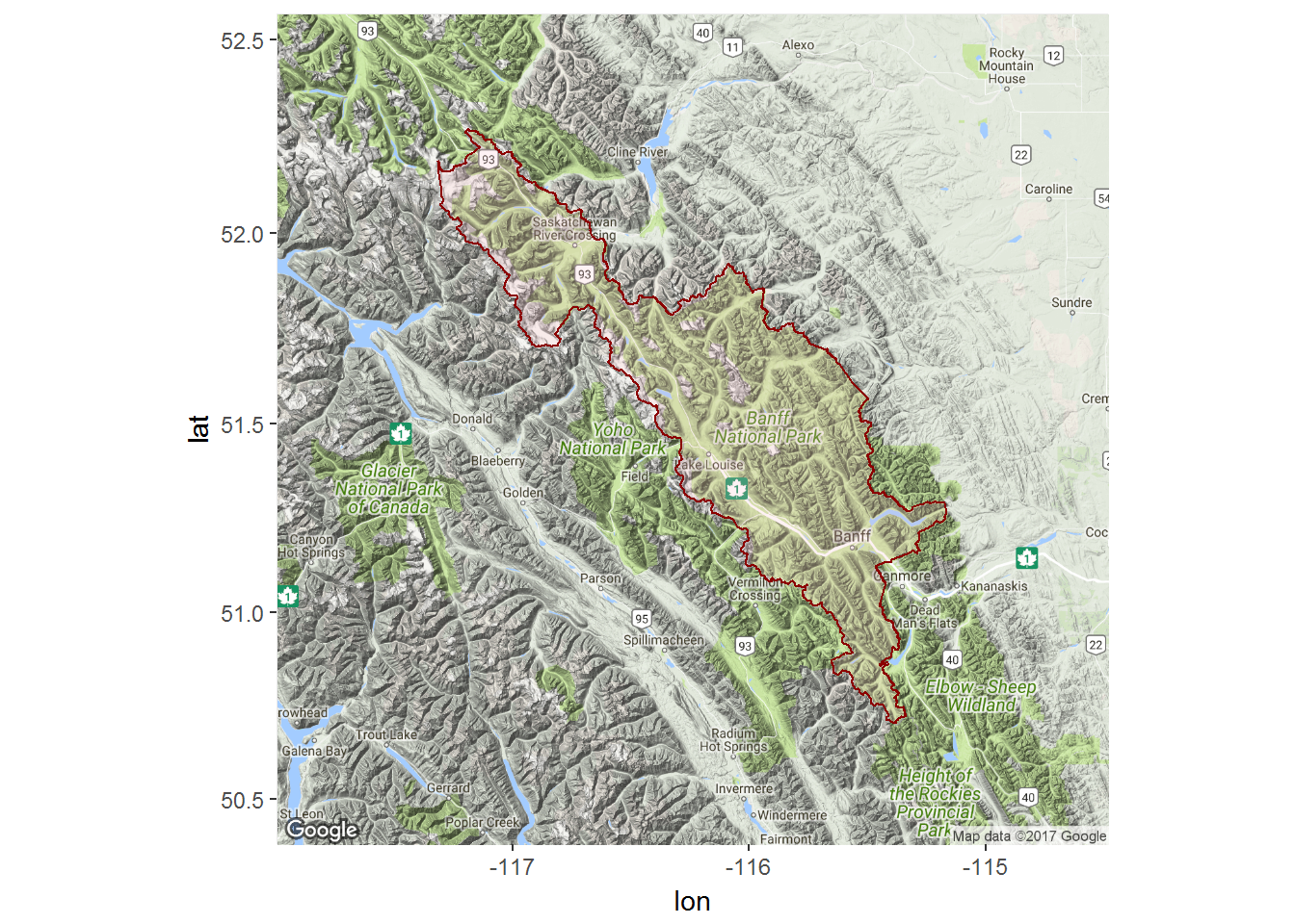
Loading rasters
Rasters are very efficient spatial matrices. They break up space into equal sized grids and store attributes at each grid point. One common way they are stored is as geoTiff objects. This link: https://terpconnect.umd.edu/~egurarie/teaching/MovementAtICCB2017/data/ should contain several rasters, notable: landcover.tif and elevation.tif. Download these to your data drive and load them.
The elevation plot is straightforward:
require(raster)
elevation <- raster("./_data/elevation.tif")
elevation
## class : RasterLayer
## dimensions : 1898, 2298, 4361604 (nrow, ncol, ncell)
## resolution : 90, 90 (x, y)
## extent : 443680.6, 650500.6, 5618416, 5789236 (xmin, xmax, ymin, ymax)
## coord. ref. : +proj=utm +zone=11 +ellps=GRS80 +towgs84=0,0,0,0,0,0,0 +units=m +no_defs
## data source : C:\Users\elie\Dropbox\teaching\ICCB-movement\lectures\_data\elevation.tif
## names : elevation
## values : 789.7076, 3571.971 (min, max)plot(elevation)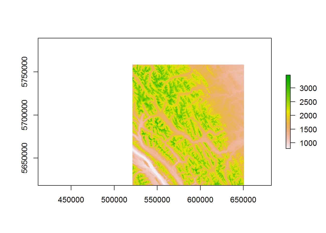
And the landcover.
landcover <- raster("./_data/landcover.tif")
landcover
## class : RasterLayer
## dimensions : 5694, 6892, 39243048 (nrow, ncol, ncell)
## resolution : 30, 30 (x, y)
## extent : 443680.6, 650440.6, 5618416, 5789236 (xmin, xmax, ymin, ymax)
## coord. ref. : +proj=utm +zone=11 +ellps=GRS80 +towgs84=0,0,0,0,0,0,0 +units=m +no_defs
## data source : C:\Users\elie\Dropbox\teaching\ICCB-movement\lectures\_data\landcover.tif
## names : landcover
## values : 0, 16 (min, max)
## attributes :
## ID category
## from: 0
## to : 16 Alpine Shrubplot(landcover)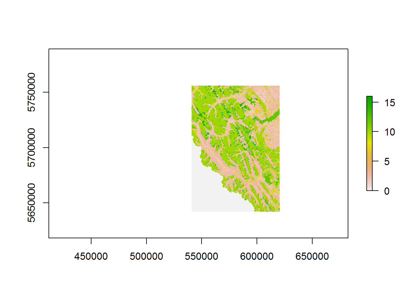
What what does 0 to 15 mean? This is a bit mysterious … it is buried here:
landcover@data@attributes## [[1]]
## ID category
## 1 0
## 2 1 Open Conifer
## 3 2 Moderate Conifer
## 4 3 Closed Conifer
## 5 4 Burn-Grassland
## 6 5 Burn-Shrub
## 7 6 Alpine Herb
## 8 7 Water
## 9 8 Deciduous
## 10 9 Mixed forest
## 11 10 Regeneration
## 12 11 Herbaceous
## 13 12 Shrub
## 14 13 Rock-Ice
## 15 14 Cloud
## 16 15 Burn-Forest
## 17 16 Alpine ShrubHere’s some quicky code to labeling the landscape layers. Note, using image is much faster (for some reason) than the raster plotting method:
landtypes <- landcover@data@attributes[[1]]
cols <- rainbow(nrow(landtypes))
cols[1] <- "white"
image(landcover, col=cols)
legend("left", legend = landtypes$category, fill = cols, bty="n", cex = 0.8)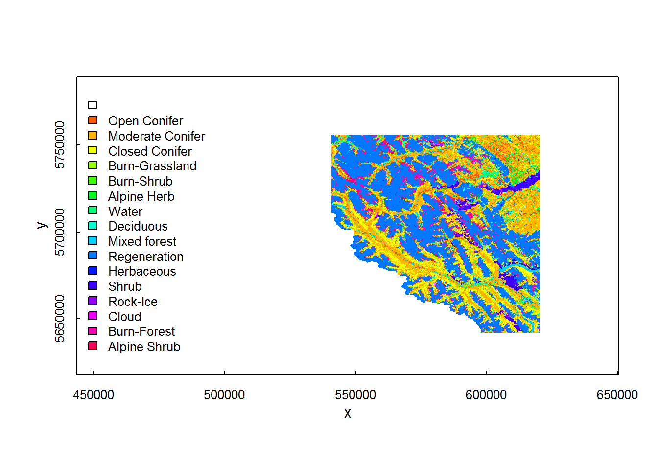
You can, of course, associate specific colors to each land cover type and add that as a column to the landtypes data frame.
Projecting
The projection of the rasters does not match the projection of our shape file:
projection(banff)## [1] "+proj=longlat +datum=WGS84 +no_defs +ellps=WGS84 +towgs84=0,0,0"projection(landcover)## [1] "+proj=utm +zone=11 +ellps=GRS80 +towgs84=0,0,0,0,0,0,0 +units=m +no_defs"projection(elevation)## [1] "+proj=utm +zone=11 +ellps=GRS80 +towgs84=0,0,0,0,0,0,0 +units=m +no_defs"No problem … we can coerce banff to match the projection we want with the spTransform() function from sp:
require(sp)
banff <- spTransform(banff, CRS(projection(landcover)))
Now, we can plot everything together:
image(elevation, col = terrain.colors(100), asp = 1, xlim =  bbox(elevation)[1,], ylim =  bbox(elevation)[2,],
            main = "elevation")
lines(banff, col="darkred", lwd=1.5)

image(landcover, col=cols, asp=1, xlim =  bbox(elevation)[1,], ylim =  bbox(elevation)[2,],
            main = "land cover")
legend("left", legend = landtypes$category, fill = cols,  cex = 0.5, bty="n")
lines(banff, col="darkred", lwd=1.5)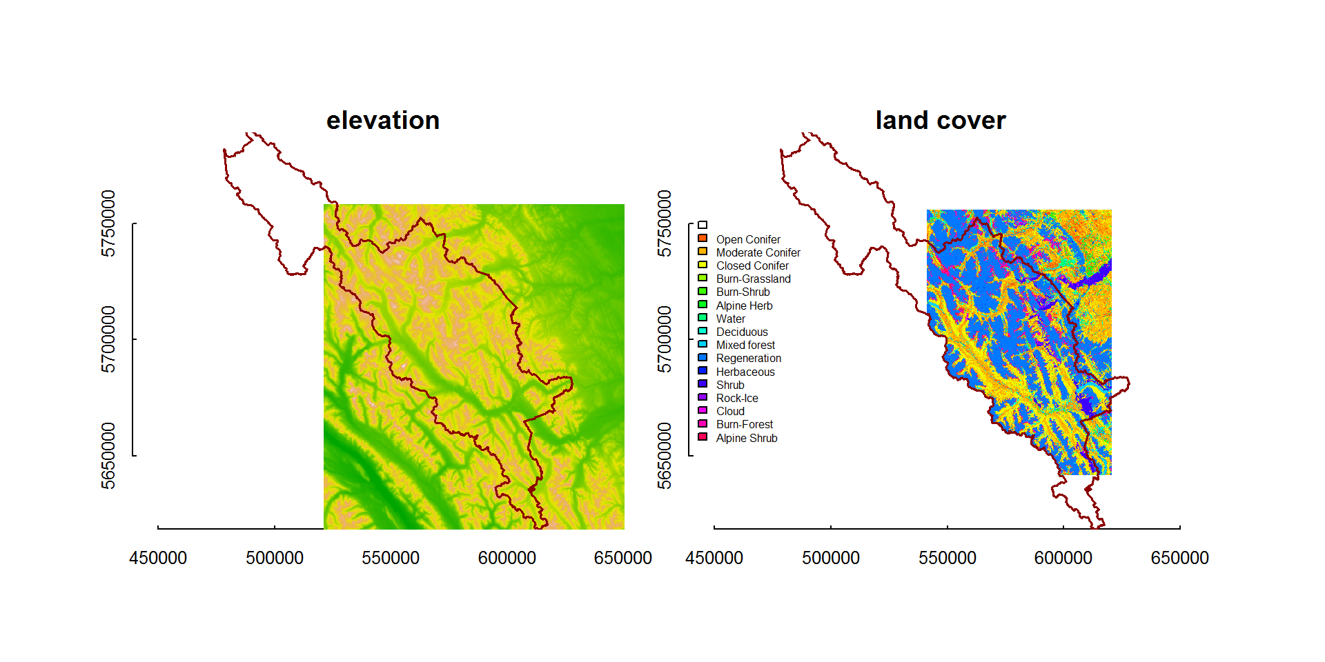
Ya Ha Tinda elk and wolf
We loaded and cleaned up data from a long-running study on elk and their predators in Alberta, Canada, the Ya Ha Tinda Elk Project. These data are made available on Movebank to anyone interested in analyzing them, thanks to Mark Hebblewhite (currently of the University of Montana).
Below is the code for loading if from movebank …
elk.study <- "Ya Ha Tinda elk project, Banff National Park (data from Hebblewhite et al. 2008)"
wolf.study <- "Ya Ha Tinda Elk Wolf (Canis lupus) project, Banff National Park, Alberta (Hebblewhite)"
elk <- getMovebankData(study=elk.study, login = login, removeDuplicatedTimestamps=TRUE)
wolf <- getMovebankData(study=wolf.study, login = login, removeDuplicatedTimestamps=TRUE)
but we will analyze cleaned up versions (as data frames) in these files:
load("./_data/elk.df.rda")
load("./_data/wolf.df.rda")

str(elk.df)
## 'data.frame': 8209 obs. of 8 variables:
## $ id : int 123288069 123288069 123288069 123288069 123288069 123288069 123288069 123288069 123288069 123288069 ...
## $ time : POSIXct, format: "2002-02-03 01:10:00" "2002-02-03 20:50:00" ...
## $ lon : num -116 -116 -116 -116 -116 ...
## $ lat : num 51.8 51.8 51.8 51.7 51.7 ...
## $ x : num 597970 598450 600359 599000 599200 ...
## $ y : num 5734300 5734500 5734295 5733600 5733400 ...
## $ temp : num NA NA NA NA NA NA NA NA NA NA ...
## $ nickname: Factor w/ 20 levels "E102","E118",..: 18 18 18 18 18 18 18 18 18 18 ...str(wolf.df)## 'data.frame': 31927 obs. of 8 variables:
## $ id : int 95424379 95424379 95424379 95424379 95424379 95424379 95424379 95424379 95424379 95424379 ...
## $ time : POSIXct, format: "2002-12-20 03:00:00" "2002-12-20 07:00:00" ...
## $ lon : num -116 -116 -116 -116 -116 ...
## $ lat : num 51.5 51.5 51.6 51.7 51.7 ...
## $ x : num 566145 566164 573124 575979 588315 ...
## $ y : num 5710864 5710819 5716322 5723442 5726959 ...
## $ temp : num -6 26 27 -5 -3 -4 24 24 28 30 ...
## $ nickname: Factor w/ 12 levels "W10","W11","W12",..: 7 7 7 7 7 7 7 7 7 7 ...Note, there are 20 elk and 12 wolves. A plot with all the animals can be a bit busy:
require(gplots)
require(plyr)

n.elk <- length(unique(elk.df$nickname))
palette(rich.colors(n.elk, alpha = 0.5))
plot(banff, main = "Elk tracks", col="grey", bor="grey")
a <- ddply(elk.df, "nickname", function(df) lines(df$x, df$y, col=df$nickname[1]))
legend("bottomleft", legend = unique(elk.df$nickname), col = 1:n.elk, lty = 1, cex = 0.5, bty="n", ncol=2)

n.wolf <- length(unique(wolf.df$nickname))
palette(rich.colors(n.wolf, alpha = 0.5))
plot(banff, main = "Wolf tracks", col="grey", bor="grey")
a <- ddply(wolf.df, "nickname", function(df) lines(df$x, df$y, col=df$nickname[1]))
legend("bottomleft", legend = unique(wolf.df$nickname), col = 1:n.wolf, lty = 1, cex = 0.5, bty="n", ncol=2)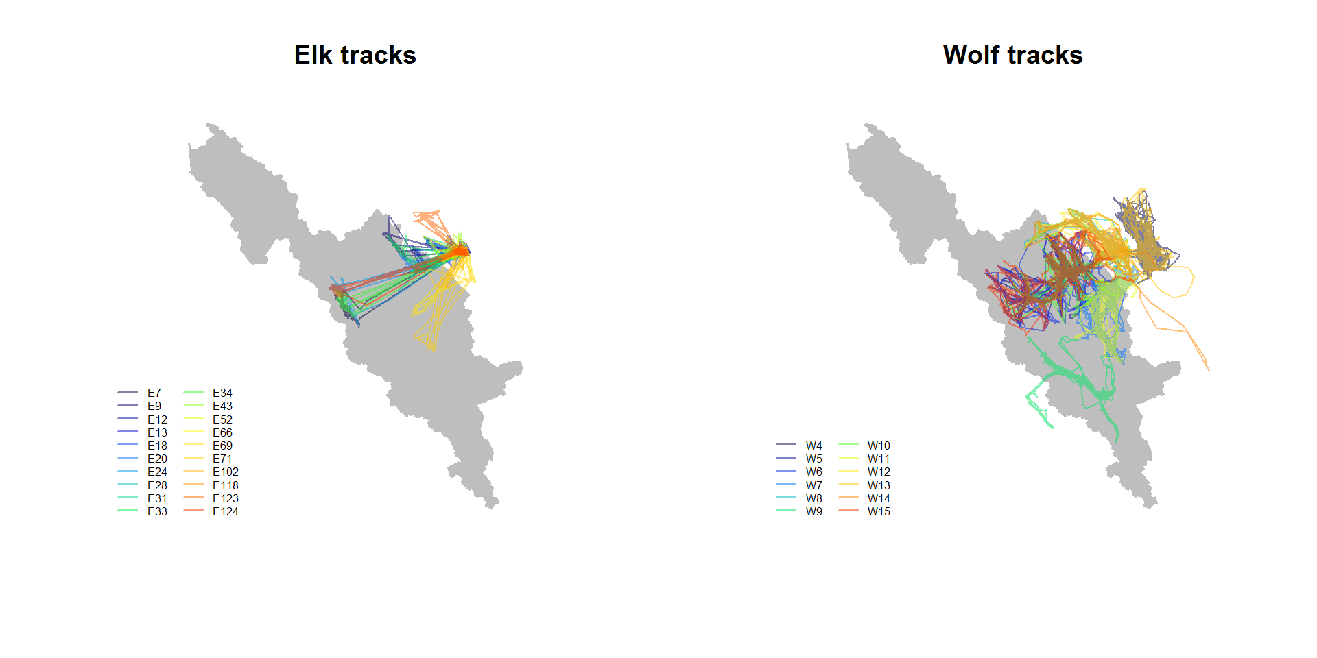
Sometimes, it can be nice to see the shape of the tracks separately:
par(mfrow = c(4,5), mar = c(0,0,3,0), oma = c(2,2,4,2))
ddply(elk.df, "nickname", function(df){
                    plot(banff, col="lightgreen", bor=NA,
                             xlim = range(df$x), ylim = range(df$y),
                             main = df$nickname[1])
                        points(df$x, df$y, col = alpha("black",.2),
                                     type="o", pch = 19, cex = 0.5)})
## data frame with 0 columns and 0 rowstitle("Elk tracks", outer = TRUE)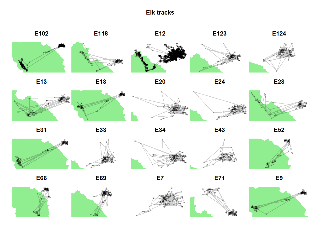
par(mfrow = c(3,4), mar = c(0,0,5,0), oma = c(2,2,4,2))
ddply(wolf.df, "nickname",
            function(df){
                    plot(banff, col="lightgreen", bor=NA,
                             xlim = range(df$x), ylim = range(df$y),
                             main = df$nickname[1]); box()
                    points(df$x, df$y, col = alpha("black",.2),
                                 type="o", pch = 19, cex = 0.5)})
## data frame with 0 columns and 0 rowstitle("Wolf tracks", outer = TRUE)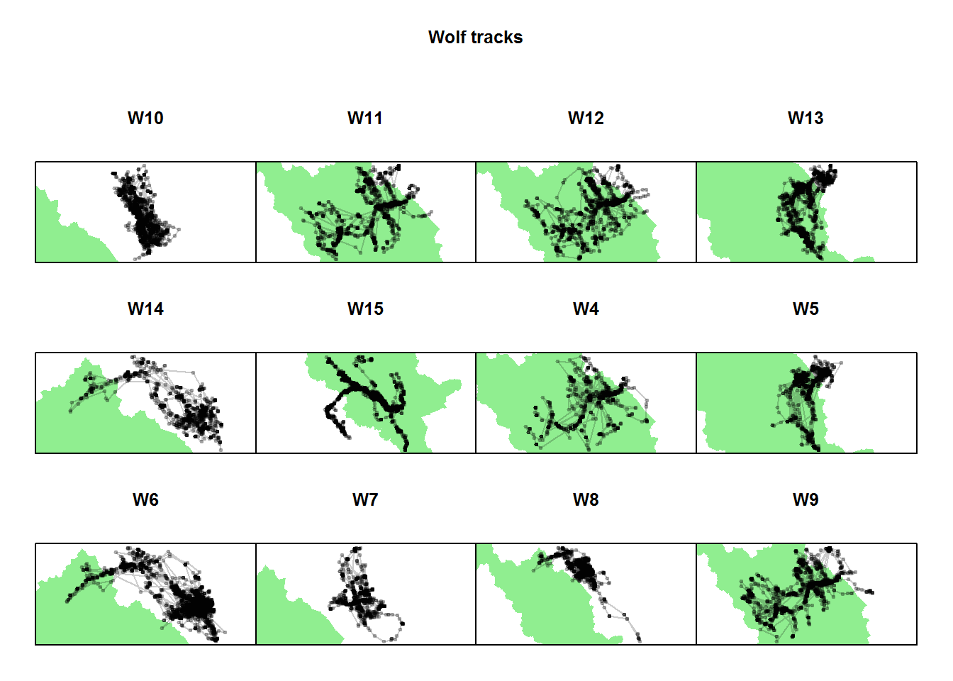
Home ranges and MCP’s
There is a an extensive and complex literarure on what constitites a “home range”. Of relatively recent note are definitions provided by Brownian Bridges (see Kranstauber) and auto-correlated kernel density estimates (akde’s) (see Fleming and Calabrese and co.)
The simplest definition - by far - is the minimum convex polygon, which simply takes observations and draws a tight polygon around the points. This is a problematic definition, but redeemed somewhat by its incredible simplicity.
Here is how to compute the MCP’s usign the adehabtitatHR package, focussing on one elk:
require(adehabitatHR)

# extact one elk, convert "xy" to  Spatial Points object

myelk <- subset(elk.df, nickname == "E102")
xy.spatial <- SpatialPoints(myelk[,c("x","y")])
myelevation <- crop(elevation, extent(xy.spatial))

# plot elevations and line

image(myelevation, asp=1, col=terrain.colors(100))
with(myelk,
points(x,y, type="o", pch = 19, cex = 0.5, col=rgb(0,0,0,.2)))

# the key command:
myelk.mcp <- mcp(xy.spatial, 100)
lines(myelk.mcp, col = "red", lwd=2)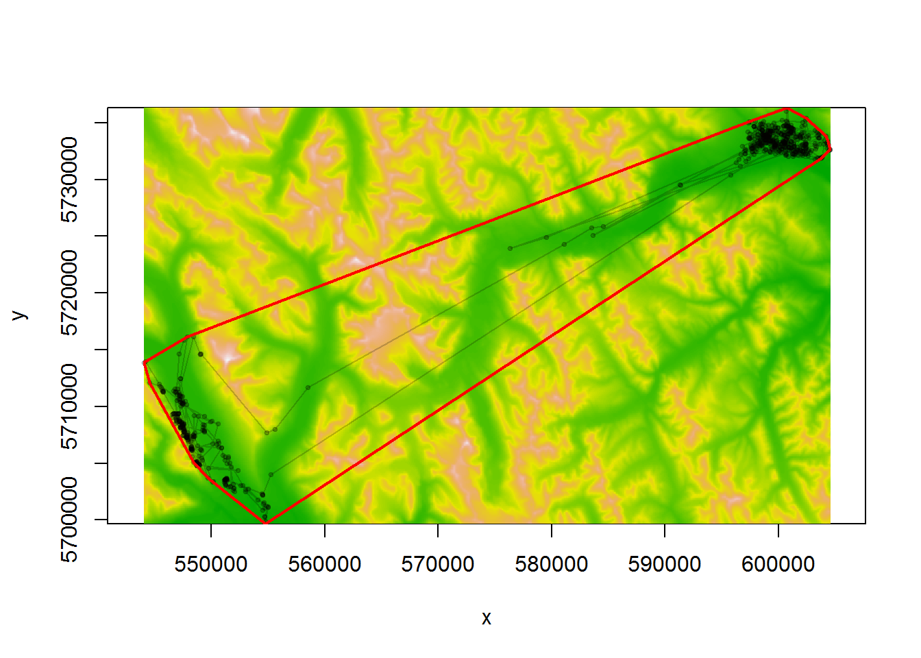
myelk.mcp## Object of class "SpatialPolygonsDataFrame" (package sp):
##
## Number of SpatialPolygons: 1
##
## Variables measured:
## id area
## a a 72630.98Lets also get some random points from within the MCP. The key function: spsample:
random.points <- spsample(myelk.mcp, 1000, "random")
image(myelevation, col = terrain.colors(100), asp=1)
lines(banff, col="white", lwd=2)
points(random.points, col=rgb(1,1,1,alpha = 0.5), pch = 19, cex=0.5)
lines(myelk.mcp, col="red", lwd=2)
points(myelk$x, myelk$y, type="o", cex=0.5, col= rgb(0,0,0,.5), pch = 19)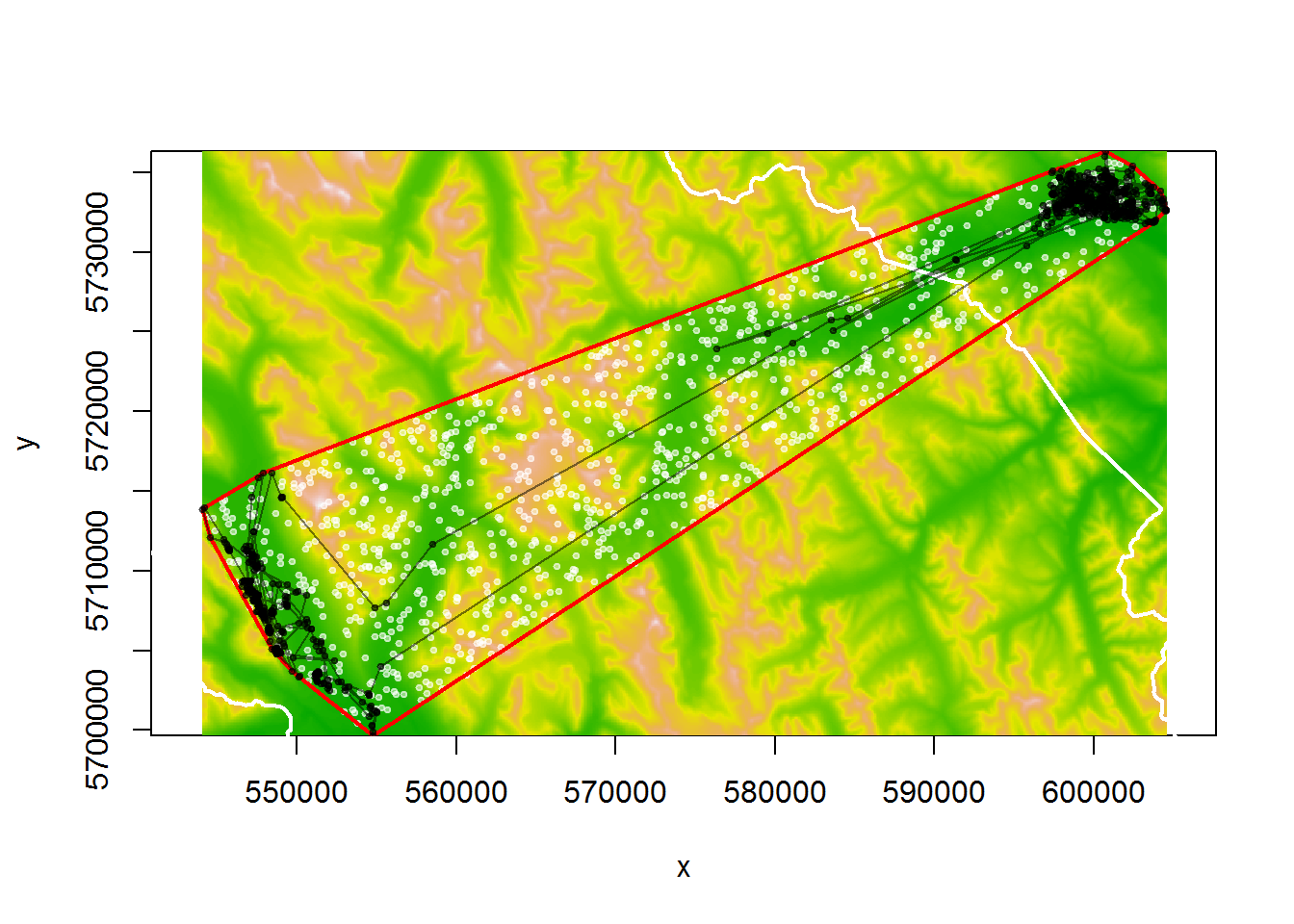
This will be useful later
Extracting spatial variables
The first step in analyzing a movement with respect ot covariates is finding out where the movement took place. We have several questions: (a) is it inside or outside the protected area? (b) What altitudes does the animal prefer? (c) What landcover is it spending the most time in?
In or out?
The basic question of how much time is (each) animal spending in or out of the park is answered with simple function.
banff.xy <- banff@polygons[[1]]@Polygons[[1]]@coords
elk.df$inout <- point.in.polygon(elk.df$x, elk.df$y, banff.xy[,1], banff.xy[,2])
plot(banff, xlim= range(elk.df$x), ylim = range(elk.df$y), col="yellow", bor = NA)
#with(elk.df, points(x, y, col = alpha(inout + 1, .2), pch = 19, cex = 0.5))
box()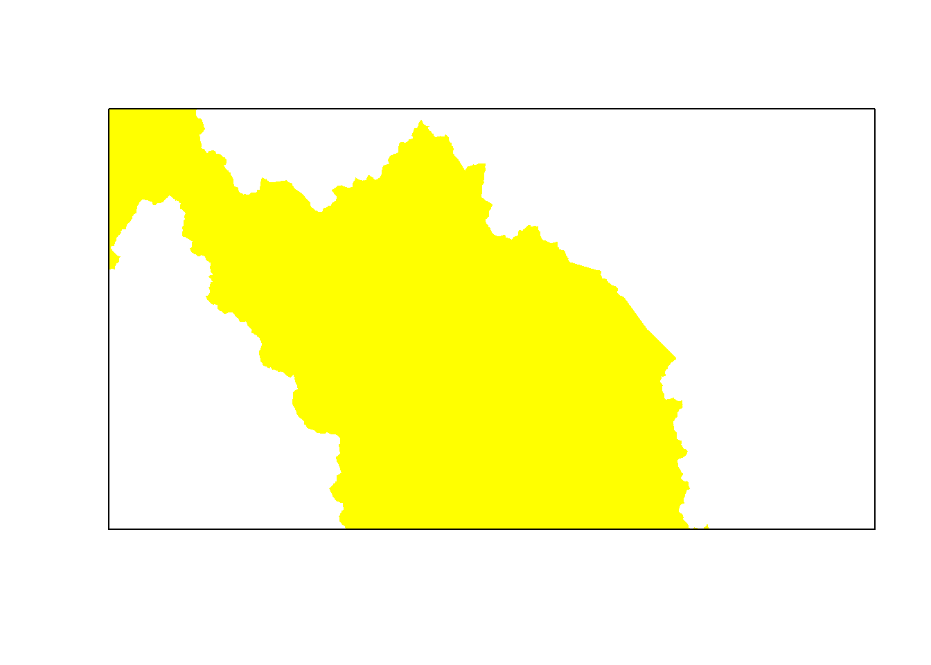
And a quick table to count the proportion of time spent in and out of the park:
ddply(elk.df, "nickname", summarize,
            n.in = sum(inout),
            n.out = sum(!inout),
            p.in = sum(inout)/length(inout))
## nickname n.in n.out p.in
## 1 E102 282 465 0.37751004
## 2 E118 26 82 0.24074074
## 3 E12 822 4722 0.14826840
## 4 E123 2 118 0.01666667
## 5 E124 0 106 0.00000000
## 6 E13 40 81 0.33057851
## 7 E18 51 80 0.38931298
## 8 E20 0 116 0.00000000
## 9 E24 0 104 0.00000000
## 10 E28 17 57 0.22972973
## 11 E31 52 70 0.42622951
## 12 E33 0 98 0.00000000
## 13 E34 0 118 0.00000000
## 14 E43 0 78 0.00000000
## 15 E52 26 46 0.36111111
## 16 E66 22 67 0.24719101
## 17 E69 8 109 0.06837607
## 18 E7 0 126 0.00000000
## 19 E71 0 100 0.00000000
## 20 E9 47 71 0.39830508Raster analysis
For rasters, all of these questions are easily answered with the extract function. It looks (from the MCP plot above) that the elk prefers moving in the valleys, which probably affects the landcover strongly as well. Let’s get the values of those elevations and compare with a couple different samplings.
xy.spatial <- SpatialPoints(myelk[,c("x","y")])
myelevation <- crop(elevation, extent(xy.spatial))
mylandcover <- crop(landcover, extent(xy.spatial))

myelk$elevation <- extract(myelevation, xy.spatial)
myelk$landcover <- extract(mylandcover, xy.spatial)

random.elevation <- extract(myelevation, random.points)
random.landcover <- extract(mylandcover, random.points)
Below - some (slightly fussy) code to visualize the difference between these samples:
# overlapping histograms
hist(myelevation, col="grey", breaks = seq(1550,3350,20), freq=FALSE, bor="darkgrey", ylim = c(0,0.01))
hist(random.elevation, col=rgb(0,1,0,.5), breaks = seq(1550,3350,30), freq=FALSE, bor="darkgrey", ylim = c(0,0.01), add=TRUE)
hist(myelk$elevation, col=rgb(1,0,0,.5), breaks = seq(1550,3350,30), freq=FALSE, add=TRUE, bor = "red")

# usage bar plot
landcover.df <- rbind(
    data.frame(type = "elk", landcover = myelk$landcover),
    data.frame(type = "mcp", landcover = as.vector(random.landcover)),
    data.frame(type = "raster", landcover = sample(as.vector(mylandcover), 1e4)))

landcover.table <- with(landcover.df, table(type, landcover))
sums <- with(data.frame(landcover.table), tapply(Freq, type, sum))

par(cex.axis = 0.7, mar = c(6,2,4,2))
barplot(landcover.table/as.vector(sums), beside = TRUE, main = "landcover", bor=NA,
                legend.text = c("landscape","mcp","elk"),
                col = c("darkgreen","lightgreen","orange"),
                args.legend = list(x = "topleft", cex = 0.8, bty="n"),
                names.arg = mylandcover@data@attributes[[1]][,2], las = 2)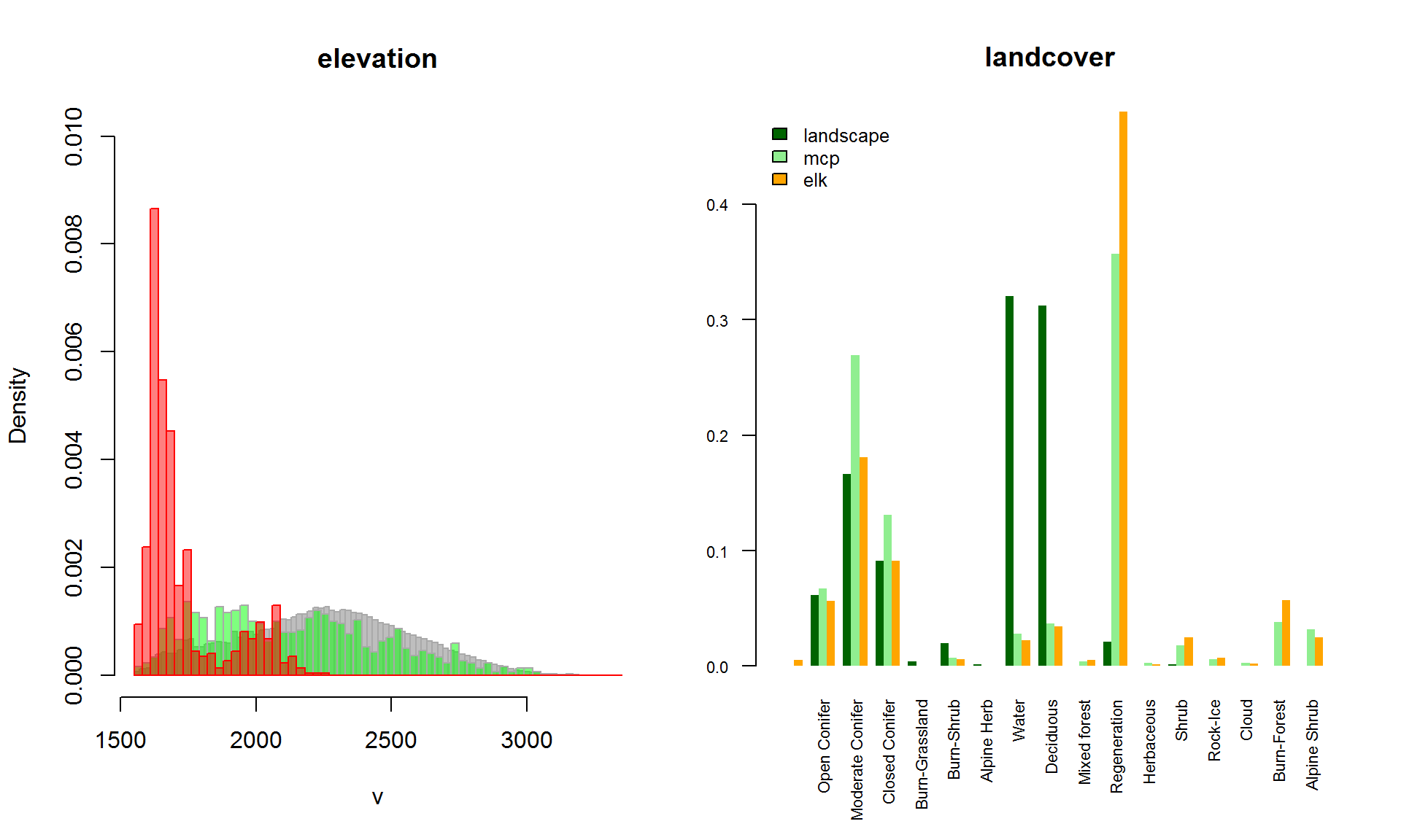
Resource Selection Functions
All the pieces are in place to do a quantitative analysis of landscape use.
Rather than analyze these data (an interesting exercise), I illustrate the process with data which are not available, but which include more variabels
deer.locs <- read.csv("rsf/deer.csv")
elevation <- raster("rsf/elevation.asc")
shrub <- raster("rsf/shrub.asc")
barren <- raster("rsf/barren.asc")
roads <- raster("rsf/rds.asc")
wells <- raster("rsf/wells.asc")
save(deer.locs, elevation, shrub, barren, roads, wells, file = "deerrasters.robj")
p <- function(alpha=0.3) points(deer.locs, cex=0.5, col=rgb(0,0,1,alpha), pch=19)
par(mfrow=c(2,3), cex.lab = 0.5, mar = c(1,1,1,1), oma = c(5,3,1,1), xpd=NA, bty="n")
plot(elevation, main = "elevation", xaxt="n", xlab=""); p()
plot(wells, main = "wells", xaxt="n", xlab="", yaxt="n", ylab=""); p()
plot(shrub, main = "shrub", xaxt="n", xlab="", yaxt="n", ylab=""); p()
plot(barren, main = "barren"); p()
plot(roads, main = "roads", yaxt="n", ylab=""); p()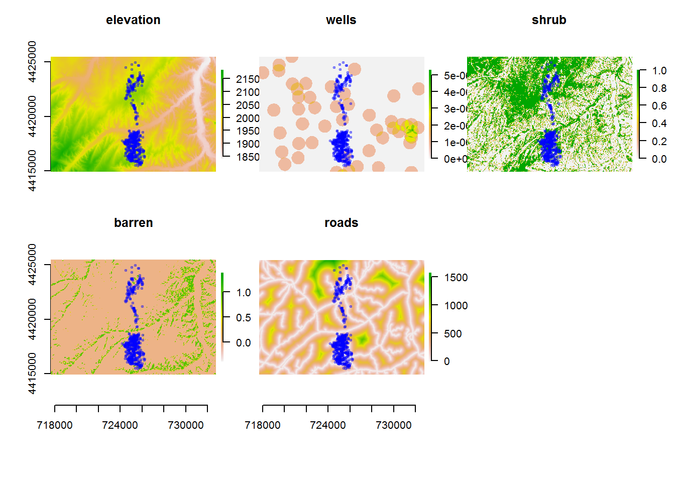
Determine available space (simplistically: MCP)
deer.mcp <- mcp(SpatialPoints(deer.locs), 100)# OLD VERSION
deer.mcp.xy <- deer.mcp@polygons[[1]]@Polygons[[1]]@coords
# FORTIYFY
require(ggplot2)
deer.mcp.xy <- fortify(deer.mcp)plot(elevation)
points(deer.locs, asp=1, pch=19, col=rgb(0,0,.4,.5), cex=0.5)
lines(deer.mcp, col="darkred", lwd=2)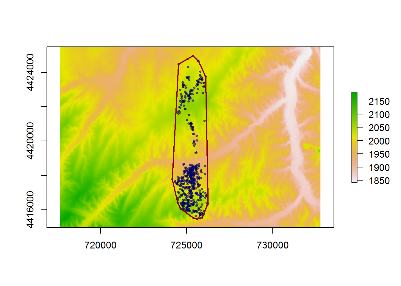
Create data frame of covariates
deer.sp<-SpatialPoints(deer.locs)

used.df <- data.frame(
  used = rep(1, length(deer.sp)),
  elevation = extract(elevation, deer.sp),
  shrub = ceiling(extract(shrub, deer.sp)),
  barren = ceiling(extract(barren, deer.sp)),
  wells = ceiling(extract(wells, deer.sp)),
  roads = ceiling(extract(roads, deer.sp)))

head(used.df)
## used elevation shrub barren wells roads
## 1 1 2052.134 1 0 1 180
## 2 1 2050.978 1 0 1 130
## 3 1 2039.769 0 0 0 434
## 4 1 2044.926 1 0 0 308
## 5 1 2010.022 1 0 0 114
## 6 1 2023.509 1 0 0 7Obtain some random points within mcp
random.points <- spsample(deer.mcp, 1000, "random")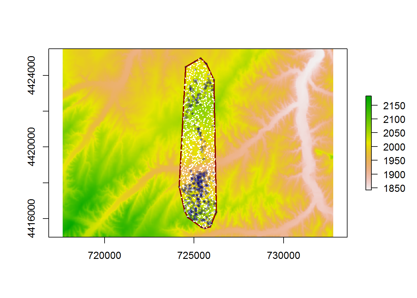
Calculate the covariates for the null set
avail.df <- data.frame(
  used = rep(0, length(random.points)),
  elevation = extract(elevation, random.points),
  shrub = ceiling(extract(shrub, random.points)),
  barren = ceiling(extract(barren, random.points)),
  wells = ceiling(extract(wells, random.points)),
  roads = ceiling(extract(roads, random.points)))

head(avail.df)
## used elevation shrub barren wells roads
## 1 0 2011.771 0 1 1 300
## 2 0 2045.179 0 0 1 311
## 3 0 2042.456 0 0 1 117
## 4 0 2024.239 1 1 0 35
## 5 0 2026.607 1 0 0 181
## 6 0 2021.193 1 0 0 70Combine…
deer.data <- rbind(avail.df, used.df)
with(deer.data, table(used, barren))
## barren
## used 0 1
## 0 910 90
## 1 494 31… and Model!
Simplest imaginable logistic regression model:
s <- function(x) x/sd(x)
deer.rsf <- glm(used ~ barren + shrub + s(elevation) + s(roads) + s(wells), family="binomial",
                data = deer.data)
## Estimate Std. Error z value P.value
## (Intercept) -9.48537776 3.73886523 -2.5369670 0.011
## barren -0.42163808 0.22509091 -1.8731902 0.061
## shrub 0.08318171 0.12469271 0.6670936 0.505
## s(elevation) 0.14407110 0.06074930 2.3715679 0.018
## s(roads) 0.10417756 0.05582293 1.8662144 0.062
## s(wells) -0.25187228 0.06024763 -4.1806174 0.000Model Selection
For intense model selection …. Dredge!
#install.packages("MuMIn")
require(MuMIn)
options(na.action = "na.fail")
deer.dredge <- dredge(deer.rsf)
deer.rsf <- glm(used ~ shrub * barren * elevation, family="binomial", data = deer.data)
deer.dredge <- dredge(deer.rsf)
head(deer.dredge)
## Global model call: glm(formula = used ~ shrub * barren * elevation, family = "binomial",
## data = deer.data)
## ---
## Model selection table
## (Int) brr elv shr brr:elv brr:shr elv:shr brr:elv:shr
## 39 -29.93 0.01444 35.10 -0.01730
## 40 -28.22 -0.2068 0.01361 33.72 -0.01663
## 48 -26.55 -15.7500 0.01278 32.61 0.007783 -0.01608
## 56 -27.87 -0.2529 0.01344 33.29 0.08803 -0.01643
## 64 -26.03 -16.2100 0.01253 32.02 0.007981 0.13060 -0.01580
## 128 -27.08 -6.9670 0.01305 33.34 0.003359 -16.92000 -0.01645 0.008533
## df logLik AICc delta weight
## 39 4 -969.899 1947.8 0.00 0.440
## 40 5 -969.483 1949.0 1.18 0.244
## 48 6 -968.984 1950.0 2.20 0.147
## 56 6 -969.465 1951.0 3.16 0.091
## 64 7 -968.944 1952.0 4.14 0.056
## 128 8 -968.796 1953.7 5.86 0.023
## Models ranked by AICc(x)Top model:
deer.rsf <- glm(used ~ barren + elevation + shrub +
                         barren*(elevation +  shrub) + elevation:shrub,
                       family="binomial", data = deer.data)
Predict from model
deer.rsf <- glm(used ~ barren + elevation + shrub + roads + wells,
                       family="binomial", data = deer.data)
coefs <- deer.rsf$coef
rsf<-exp(elevation*coefs["elevation"] + roads*coefs["roads"] + wells*coefs["wells"] +
           shrub*coefs["shrub"] + barren*coefs["barren"])
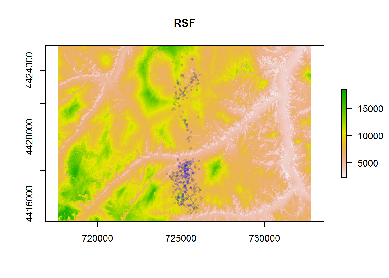
plot(rsf, main = "RSF"); p(alpha = 0.1)