Processing Movement Data
Elie Gurarie and Silvia Alvarez
August 29 - 2016
1 Preamble
Processing data is the least loved and often most time consuming aspect of any data analysis. It is also unavoidable and extremely important. There are several tools - including some more recent R packages that greatly facilitate the processing of data.
Some broad guidelines of smart data processing include:
- compartamentalized - e.g. each step a function
- interactive - leverage visualization and interactive tools
- generalizable - to apply to multiple individuals
- replicable - important: NEVER overwrite the raw data!
- well-documented - so you don’t have to remember what you did
- forgettable! - so once its done you don’t need to think about it any more
2 Packages and functions
Several packages are particularly useful for data processing:
plyr- manipulating data frames and lists- functions:
mutate;ddply-ldply-dlply lubridate- manipulating time objectsrgdal- projecting coordinatesmapsandmapdata- quick and easy mapsmagrittr- for piping
Sneaky R trick: For loading a lot of packages - makes a list:
pcks <- list('plyr', 'lubridate', 'ggmap', 'maptools', 'rgdal', 'maps', 'mapdata')and then “apply” the require function to the list:
sapply(pcks, require, character = TRUE)## [1] TRUE TRUE TRUE TRUE TRUE TRUE TRUE3 Loading Data
Load the following moose study from Movebank:
moose <- getMovebankData(study="ABoVE: Peters Hebblewhite Alberta-BC Moose", login = login)Convert to a data frame:
moose.df <- as.data.frame(moose)4 Data processing
4.1 Renaming columns
Movebank data comes with a set of (mostly) standard column names:
str(moose.df)## 'data.frame': 52356 obs. of 17 variables:
## $ external_temperature : num -9.5 -11.1 -13.7 -12.9 -15.4 ...
## $ gps_fix_type : int 3 3 3 3 3 3 3 3 3 3 ...
## $ gps_hdop : num 3.6 1.5 2 1.9 5.3 1.1 1.5 1.2 2.1 1.4 ...
## $ gps_satellite_count : int 7 9 4 2 2 10 3 3 11 4 ...
## $ gps_time_to_fix : num 51 39 82 40 39 40 40 47 51 62 ...
## $ height_above_msl : num 1198 1205 1204 1203 1198 ...
## $ location_lat : num 54.6 54.6 54.6 54.6 54.6 ...
## $ location_long : num -120 -120 -120 -120 -120 ...
## $ manually_marked_outlier: Factor w/ 2 levels "","true": 1 1 1 1 1 1 1 1 1 1 ...
## $ mw_activity_count : num 80 927 95 877 778 ...
## $ timestamp : POSIXct, format: "2009-03-08 01:02:52" "2009-03-08 03:02:40" ...
## $ update_ts : Factor w/ 1 level "1970-01-01 00:00:00.000": 1 1 1 1 1 1 1 1 1 1 ...
## $ sensor_type_id : int 653 653 653 653 653 653 653 653 653 653 ...
## $ deployment_id : int 179222573 179222573 179222573 179222573 179222573 179222573 179222573 179222573 179222573 179222573 ...
## $ event_id : int 1691019105 1691019106 1691019107 1691019108 1691019109 1691019110 1691019111 1691019112 1691019113 1691019114 ...
## $ location_long.1 : num -120 -120 -120 -120 -120 ...
## $ location_lat.1 : num 54.6 54.6 54.6 54.6 54.6 ...The nomenclature of these columns is important and unambiguous for movebank database purposes, bot for the purposes of our own analyses the column names a bit long and unwieldly. Also - a lot of the data is not that interesting or important (though note the - always interesting - temperature sensor!). We might simplify the data to a data frame that is more friendly:
moose2 <- with(moose.df, data.frame(id = deployment_id, lon = location_long, lat = location_lat, time = timestamp, Temp = external_temperature))Note - it’s bad form to be renaming objects the same name as before, which is why I called this moose2. It’s also not great form to have a whole bunch of moose1-2-3’s, because that’s confusing. We’ll see later how to combine all the data processing into a single command.
Note that the moose ID’s are long strings of numbers. That is a little awkward - for one thing they should be discrete factors, for another, it is hard to remember which moose you are actually working with. The code below adds another
n.moose <- length(unique(moose2$id))
nicknames <- paste0("M", 1:n.moose)
moose2$nickname <- factor(moose2$id, labels = nicknames)
4.2 Dates and Times
One of the scourges of movement data is dates and times, which are complicated and poorly stacked for a whole bunch of reasons related to inconsistent formatting, days and weeks and months not dividing nicely into years, etc.
The getMovebankData function (and, presumably, the Movebank database) nicely formats the times as POSIX - a standard universal data format for dates and times. If you are loading your data from a spreadsheet (e.g. via read.csv), you will have to convert the character strings into POSIX (otherwise they are loaded as factors). As an example, here is a sample of a text file containing short-toed eagle movement data:
##         Date  Time Latitude.N. Longitude.E. Speed Course Altitude.m.
## 1 2010-07-19 15:00    40.35500     18.17217     0    272         103
## 2 2010-07-19 16:00    40.35467     18.17233     0    329          95
## 3 2010-07-19 17:00    40.35483     18.17233     0    246          90
## 4 2010-08-09 07:00     0.00000      0.00000     0    124          27
## 5 2010-08-09 09:00     0.00000      0.00000     0     92          27
## 6 2010-08-09 11:00     0.00000      0.00000     0     96          27
## 'data.frame': 881 obs. of 7 variables:
## $ Date : Factor w/ 115 levels "2010-07-19","2010-08-09",..: 1 1 1 2 2 2 3 3 3 4 ...
## $ Time : Factor w/ 24 levels "00:00","01:00",..: 16 17 18 8 10 12 14 16 18 14 ...
## $ Latitude.N. : num 40.4 40.4 40.4 0 0 ...
## $ Longitude.E.: num 18.2 18.2 18.2 0 0 ...
## $ Speed : int 0 0 0 0 0 0 0 0 0 0 ...
## $ Course : int 272 329 246 124 92 96 126 104 96 290 ...
## $ Altitude.m. : int 103 95 90 27 27 27 591 27 27 647 ...To convert the Date and Time into a POSIX object, you used to have to muck around with the as.POSIX commands R which could be quite clunky.
head(as.POSIXlt(paste(eagle$Date, eagle$Time), format = "%Y-%m-%d %H:%M", tz = "UTC"))## [1] "2010-07-19 15:00:00 UTC" "2010-07-19 16:00:00 UTC"
## [3] "2010-07-19 17:00:00 UTC" "2010-08-09 07:00:00 UTC"
## [5] "2010-08-09 09:00:00 UTC" "2010-08-09 11:00:00 UTC"The lubridate package can generate these objects much more quickly, without specifying the formatting. The functions ymd and hm below “intelligently” decifer the year-month-day and hour-minute formatting of the data.
require(lubridate)
head(ymd(eagle$Date) + hm(eagle$Time))
## [1] "2010-07-19 15:00:00 UTC" "2010-07-19 16:00:00 UTC"
## [3] "2010-07-19 17:00:00 UTC" "2010-08-09 07:00:00 UTC"
## [5] "2010-08-09 09:00:00 UTC" "2010-08-09 11:00:00 UTC"In our data, the format was at least the (very sensible) YYYY-MM-DD. In the US very often dates are written down as MM/DD/YYYY (and, infuriatingly, always saved that way by Excel). For lubridate … no problem:
dates <- c("5/7/1976", "10-24:1979", "1.1.2000")
mdy(dates)
## [1] "1976-05-07" "1979-10-24" "2000-01-01"One other nice feature of lubridate is the ease of getting days of year, hour or days, etc. from data, e.g.:
hour(moose2$time)[1:10]## [1] 1 3 5 7 9 11 13 15 17 19month(moose2$time)[1:10]## [1] 3 3 3 3 3 3 3 3 3 3yday(moose2$time)[1:10]## [1] 67 67 67 67 67 67 67 67 67 674.3 Quick plot
require(ggplot2)
ggplot(moose2, aes(x = lon, y = lat, col = nickname)) + geom_path()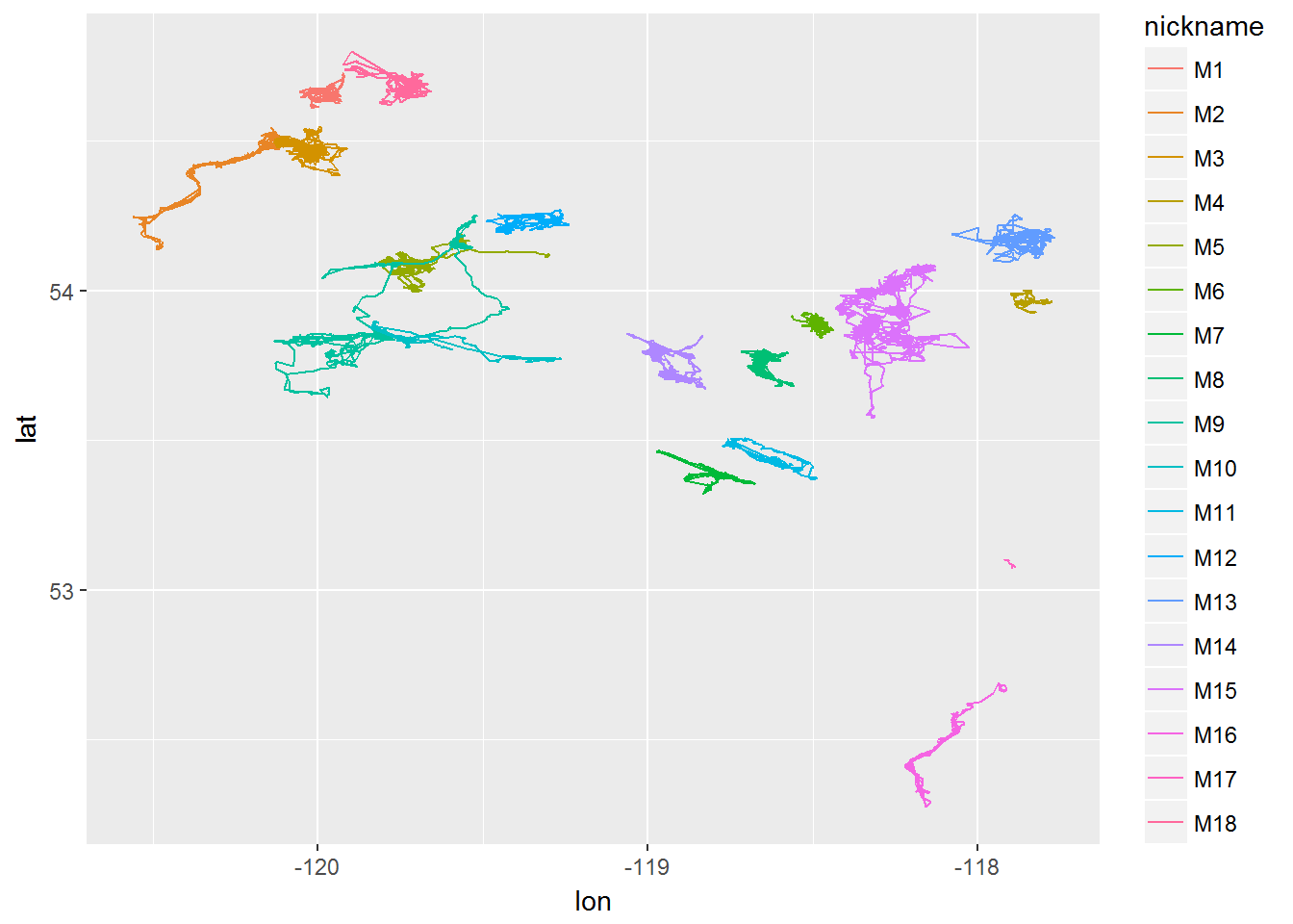
4.4 Latitudes, longitudes
It is nice to have Lat-Long data for seeing where your data are located in the world. But degrees latitude and longitude are not of consistent size, and movement statistics are best used in a consistent format, with “real” distances between points - whether in kilometers or meters.
4.4.1 … into UTM
One widely used type of projection for this purpose is “Universal transverse mercator” which will transform your data to meters north and east of one of 60 points at 6 degree intervals around the equator. One function that does this is convUL in PBSmapping. Its a bit awkward to use, as the data have to have columns names “X” and “Y” and have an “attribute” called “” “LL” so that it knows that its converting from a lat-long:
require(PBSmapping)
ll <- with(moose2, data.frame(X = lon, Y = lat))
attributes(ll)$projection <- "LL"
xy.km <- convUL(ll, km=TRUE)
head(xy.km)
## X Y
## 1 306.6212 6055.973
## 2 306.5993 6055.972
## 3 306.6085 6055.959
## 4 306.5622 6055.936
## 5 306.5792 6055.903
## 6 306.6119 6055.899Note that the function determined that the best zone for these data would be zone 11. That is an easy variable to change. We can now say (roughly) that the total extent of the moose movements was in kilometers:
diff(range(xy.km$X))## [1] 181.8704diff(range(xy.km$Y))## [1] 283.8164So over 3700 km north-south, and 2000 km east-west. You can add this to the moose data frame:
moose3 <- data.frame(moose2, x=xy.km$X, y=xy.km$Y)4.4.2 … using proj4
All projections (including) comprehensive projection standard is the PROJ4 system, which GIS users should be aware of. In particular when you are working with spatial files from other sources (e.g. habitat layers, bathymetry models), you need to make sure that your coordinates match up.
The original movebank loaded moose object is an even more complex version of an SpatialPointsDataFrame object, itself a somewhat complex spatial data object:
is(moose)## [1] "MoveStack" ".MoveTrackStack"
## [3] ".MoveGeneral" ".MoveTrack"
## [5] ".unUsedRecordsStack" "SpatialPointsDataFrame"
## [7] ".unUsedRecords" "SpatialPoints"
## [9] "Spatial" "SpatialVector"Its projection is:
moose@proj4string## CRS arguments:
## +proj=longlat +ellps=WGS84 +datum=WGS84 +towgs84=0,0,0We can reproject the moose into any other projection, for example the UTM zone 11 projection (which you can look up here: http://www.spatialreference.org/ref/epsg/wgs-84-utm-zone-11n/) has the following proj4 code: +proj=utm +zone=11 +ellps=WGS84 +datum=WGS84 +units=m +no_defs
The function that re-projects these data is spTransform
require(rgdal)
projection <- CRS("+proj=utm +zone=11 +ellps=WGS84 +datum=WGS84 +units=m +no_defs ")
moose.projected <- spTransform(moose, projection)
plot(moose.projected)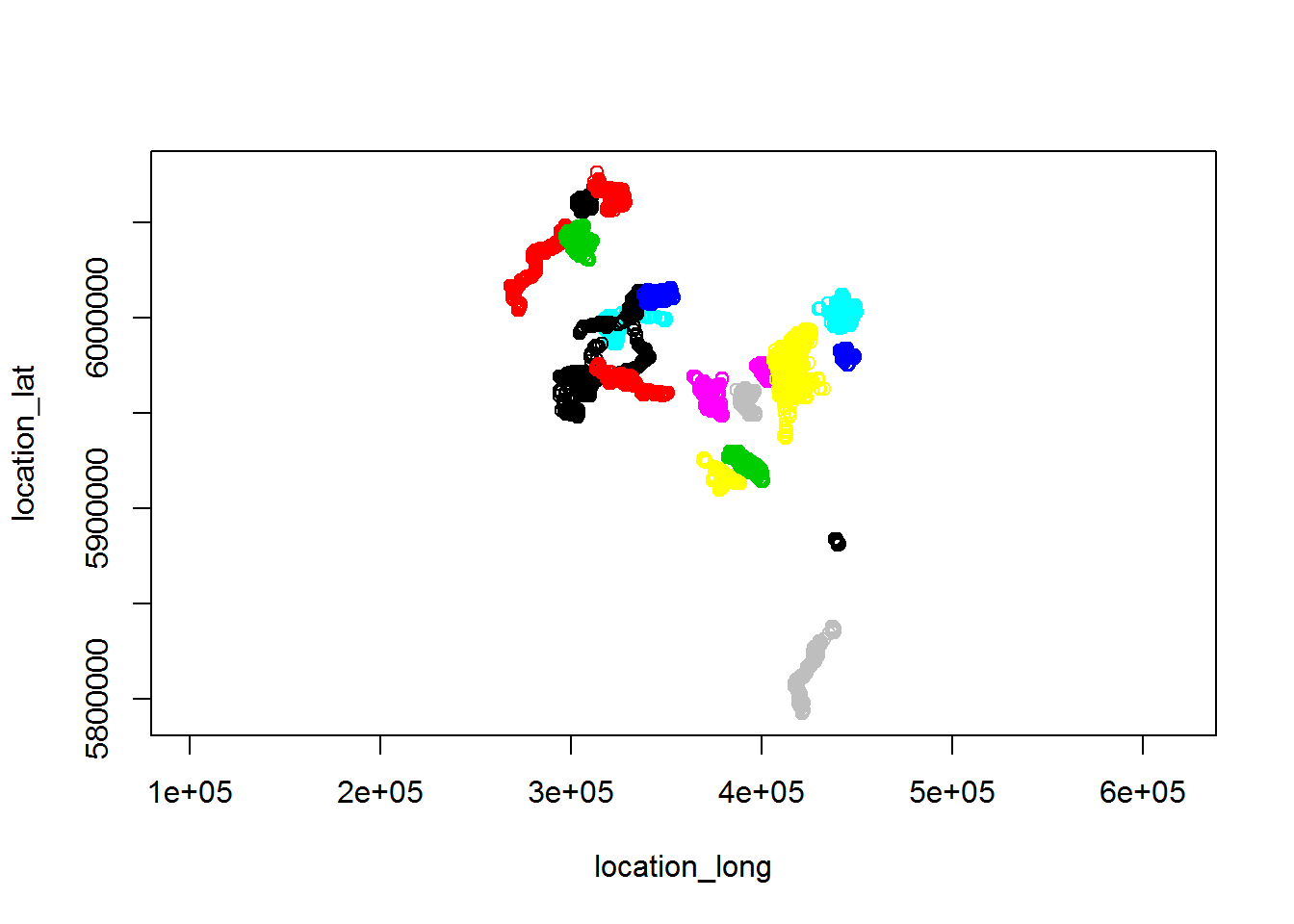
We can extract the x,y coordinates (as above) by converting to a data frame:
moose.projected.df <- data.frame(moose.projected)
names(moose.projected.df)
## [1] "external_temperature" "gps_fix_type"
## [3] "gps_hdop" "gps_satellite_count"
## [5] "gps_time_to_fix" "height_above_msl"
## [7] "location_lat" "location_long"
## [9] "manually_marked_outlier" "mw_activity_count"
## [11] "timestamp" "update_ts"
## [13] "sensor_type_id" "deployment_id"
## [15] "event_id" "location_long.1"
## [17] "location_lat.1" "optional"Two new columns were added to the data frame: location_long.1 and location_lat.1 - there are the projected data.
xy.projected <- moose.projected.df[,c("location_long.1", "location_lat.1")]A quick test to see if the two projections agree:
diff(range(xy.km[,1]))## [1] 181.8704diff(range(xy.projected[,1]))/1000## [1] 181.8704diff(range(xy.km[,2]))## [1] 283.8164diff(range(xy.projected[,2]))/1000## [1] 283.8164Excellent. So either method will work.
5 Summaries
require(plyr)
ddply(moose3, "nickname", summarize,
            n.obs = length(nickname),
            start = as.Date(min(time)),
            end = as.Date(max(time)),
            duration = max(time) - min(time),
            median.Dt = median(diff(time)),
            range.x = diff(range(x)),
            range.y = diff(range(y)))
## nickname n.obs start end duration median.Dt
## 1 M1 4019 2009-03-08 2010-02-20 349.91743 days 2.000000 hours
## 2 M2 4086 2009-03-08 2010-02-16 345.91635 days 2.000000 hours
## 3 M3 1785 2008-03-13 2009-01-20 313.83346 days 4.000000 hours
## 4 M4 1534 2008-03-12 2009-02-10 335.83332 days 4.000000 hours
## 5 M5 4105 2009-03-08 2010-02-18 347.91668 days 2.000000 hours
## 6 M6 4083 2009-03-09 2010-02-18 346.91649 days 2.000000 hours
## 7 M7 1705 2008-12-04 2010-02-18 441.33332 days 4.000000 hours
## 8 M8 1831 2008-03-14 2009-01-21 313.83306 days 4.000000 hours
## 9 M9 4151 2009-03-08 2010-02-19 348.91693 days 2.000000 hours
## 10 M10 2640 2008-12-05 2010-02-28 450.83370 days 4.000000 hours
## 11 M11 2052 2008-12-04 2010-02-19 442.66666 days 4.000000 hours
## 12 M12 4032 2009-03-08 2010-02-18 347.91662 days 2.000000 hours
## 13 M13 1722 2008-03-12 2009-01-30 324.83398 days 4.000000 hours
## 14 M14 2603 2008-12-04 2010-02-19 442.83332 days 4.000000 hours
## 15 M15 2935 2009-03-09 2010-02-19 347.91685 days 2.000833 hours
## 16 M16 4212 2009-03-09 2010-03-09 365.91692 days 2.000000 hours
## 17 M17 860 2009-03-08 2009-05-21 74.40031 days 2.000000 hours
## 18 M18 4001 2009-03-08 2010-02-17 346.58339 days 2.000000 hours
## range.x range.y
## 1 9.185101 12.696908
## 2 31.183415 44.063304
## 3 14.434006 18.213924
## 4 8.231451 8.508530
## 5 33.944978 21.069068
## 6 8.377864 9.499633
## 7 19.702933 16.647610
## 8 10.276187 14.037471
## 9 47.476258 66.389747
## 10 37.871944 16.357794
## 11 18.698625 15.752861
## 12 16.208209 8.511487
## 13 20.166264 17.566005
## 14 15.252216 20.895569
## 15 26.481225 57.101170
## 16 21.335886 45.495071
## 17 2.260760 3.126237
## 18 17.001690 20.238892Visualize temporal extent of data:
ggplot(moose2, aes(x = time, y = nickname)) + geom_path()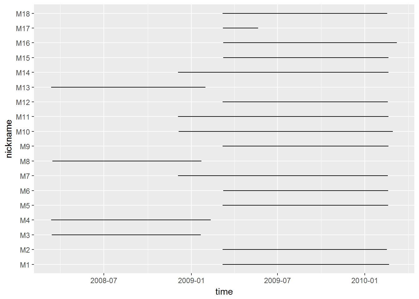
5.1 Aggregation
For some questions (e.g. major range shifts or migrations) we might not be interested in sub-daily processes. Also - the fact that the observation interals are not entirely consistent can be annoying. With ddply, it is easy to obtain, for example, a mean daily location. But first you need to obtain the day of each location
moose3$day.date <- as.Date(moose3$time)moose4<- ddply(moose3, c("id", "day.date"), summarize,
time = mean(time),
lon = mean(lon),
lat = mean(lat),
x = mean(x), y = mean(y))This is a much leaner (and therefore faster) data set:
dim(moose3)## [1] 52356 9dim(moose4)## [1] 6103 7which, however, might contain most of the biology we are actually interested in.
6 One-step processing
As noted above, it’s bad form to be (a) renaming objects the same name as before, OR (b) also not great to have a whole bunch of moose1-2-3’s, because that’s confusing.
Super sneaky R trick: There’s a funky technique called “piping” in the package magrittr which allows you do many steps as a single step. Check out examples and documentation, but in the meantime, compare the code below with the code above. It is possible to combine almost all of these steps into a single piped command:
require(magrittr)

getUTM <- function(data){
    ll <- with(moose2, data.frame(X = lon, Y = lat))
    attributes(ll)$projection <- "LL"
    xy <- convUL(ll, km=TRUE)
    data.frame(data, x = xy$X, y = xy$Y)
}

moose.df <- (moose %>% as.data.frame %>% rename(c("deployment_id" ="id",
                                                                         location_long = "lon",
                                                                         location_lat = "lat",
                                                                         timestamp = "time",
                                                                         external_temperature = "temp")))[,c("id",'lon',"lat","time","temp")] %>%
                    mutate(nickname = factor(id, labels = paste0("M", 1:length(unique(id)))),
                                 day.date = as.Date(time)) %>% getUTM %>%
                    ddply(c("id", "nickname", "day.date"), summarize,
                          time = mean(time),
                          lon = mean(lon),
                          lat = mean(lat),
                                                  temp = mean(temp),
                          x = mean(x), y = mean(y))
7 Filtering data
Another important data processing step for movement data includes filtering. Most common types of filtering include
- removing duplicates
- filtering out outliers based on speed, location, uncertainty.
7.1 Using Movebank filtering tool
You can also apply filtering to one individual by choosing it from the animals menu on the left panel or to all individuals in the study. Select the study/animal and go to Data > Show in map. This will help you decide on some of the filtering tools. Check if there are points outside the distribution range of the species, for example. Or points that represent distances/speeds not possible for the species. An initial visual exploration can help you decide if the data needs some filtering before starting any analysis.
You can filter points manually in the editor by managing attributes. You can use less subjective methods by going to Data > Edit > Filter data > General Purpose Filter and select the type of filters that you want to apply (duplicates, specific range of values, or speed.
Speed is still experimental in Movebank but includes three different ways of estimating outliers after defining limits for speed and location error.
1.Valid anchor: If movement from record x to x+1 requires an implausible speed (> speed limit), x + 1 is considered an outlier. Then, speeed between x and x + 2 is estimated and compared with the speed limit. If higher, x + 2 is also considered an outlier and the paired test countinues with the next location until a plausible speed value is found.
Longest consistent track: Finds the longest sequence of points in the track that is consistent with the speed limits you set. It starts separate tracks when a record doesn’t pass the speed limit compared to the previous record.
Simple outlier: Compares each record against previous and next records and marks it as outlier if speed is higher than the limit in both cases.
Avoid methods 1 and 2 if outliers seem to occur in groups of over 2 records or starting and finishing points are outliers.
7.2 Using R to filter data
We can use the package ‘trip’ to filter by speed. It uses the single outlier approach. Here’s an example:
We load the movement data from one particular tapir (we’ll call her Lucy) into R.
require(trip)
require(lubridate)

lucy.raw <- read.csv("./_data/Tapir3.csv")
str(lucy.raw)
## 'data.frame': 636 obs. of 16 variables:
## $ event.id : num 3.4e+09 3.4e+09 3.4e+09 3.4e+09 3.4e+09 ...
## $ visible : Factor w/ 1 level "true": 1 1 1 1 1 1 1 1 1 1 ...
## $ timestamp : Factor w/ 636 levels "2006-09-13 03:29:00.000",..: 1 2 3 4 5 6 7 8 9 10 ...
## $ location.long : num -75.5 -75.5 -75.5 -75.5 -75.5 ...
## $ location.lat : num 4.73 4.73 4.73 4.73 4.72 ...
## $ gps.dop : num 1.4 3.3 5.1 9.1 2.2 8 4.7 5 2.9 4.7 ...
## $ gps.time.to.fix : num 1 33 54 56 73 80 53 76 64 55 ...
## $ height.above.msl : num 2943 2943 0 0 0 ...
## $ sensor.type : Factor w/ 1 level "gps": 1 1 1 1 1 1 1 1 1 1 ...
## $ individual.taxon.canonical.name: Factor w/ 1 level "Tapirus pinchaque": 1 1 1 1 1 1 1 1 1 1 ...
## $ tag.local.identifier : Factor w/ 1 level "3(5TH-1360)-Tag": 1 1 1 1 1 1 1 1 1 1 ...
## $ individual.local.identifier : Factor w/ 1 level "3(5TH-1360)": 1 1 1 1 1 1 1 1 1 1 ...
## $ study.name : Factor w/ 1 level "Mountain tapir, Colombia": 1 1 1 1 1 1 1 1 1 1 ...
## $ utm.easting : num 448109 448004 448073 448129 448003 ...
## $ utm.northing : num 522585 522340 522329 522350 521888 ...
## $ utm.zone : Factor w/ 1 level "18N": 1 1 1 1 1 1 1 1 1 1 ...lucy <- with(lucy.raw, data.frame(time = ymd_hms(timestamp), x = utm.easting, y = utm.northing, id=individual.local.identifier)) We can see from an image that there are a few possible observation errors (unrealistic points).
with(lucy, plot(x, y, type="o", asp=1, col = rgb(0,0,0,.5), pch = 19, cex = 0.5, main = "Lucy")) 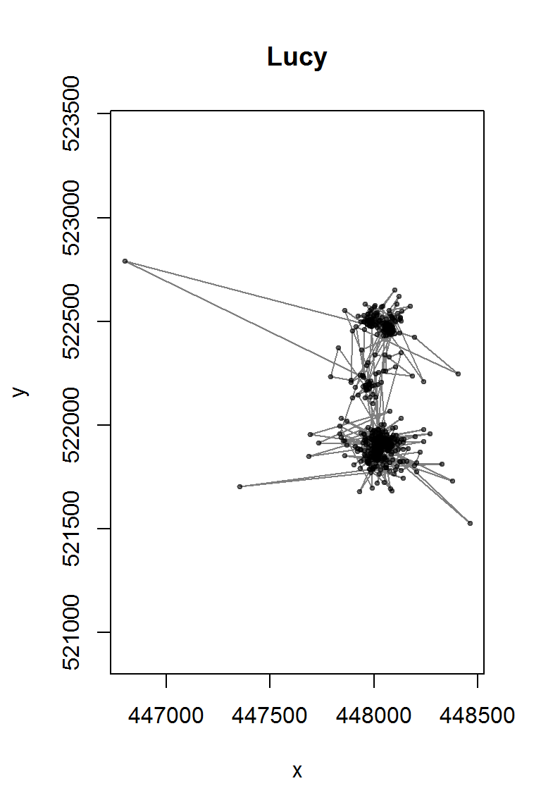
There are a few duplicated time points, which we need to filter away (note the base function duplicated):
lucy <- subset(lucy, !duplicated(time)) In order to run the filter, we need to convert the tapir to a special data type called a SpatialPointsDataFrame. The easiest (if unintuitive) way to do this is to run the coordinates() command (from package sp).
coordinates(lucy) <- ~ x + yWe add the correct projection:
proj4string(lucy) <- "+proj=utm +zone=18 +ellps=WGS84 +datum=WGS84 +units=m +no_defs"The trip function makes the spatial lines object ordered in time:
lucy.trip <- trip(lucy, TORnames = c("time", "id"))Now we can apply the speedfilter:
lucy.filtered <- lucy[speedfilter(lucy.trip, max.speed=0.08*3600),]

plot(lucy, col = 2)
plot(lucy.filtered, add=T)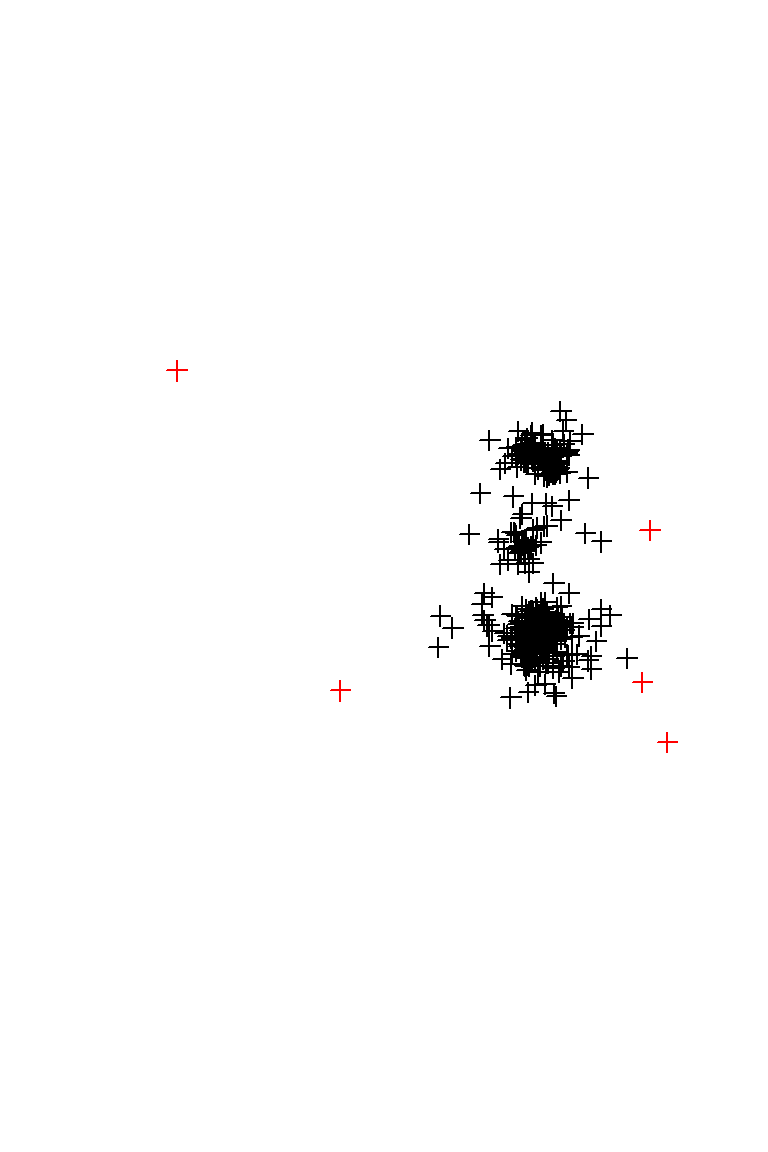
Finally, save the filtered object for later use:
save(lucy.filtered, file="./_data/TapirClean.robj")