Downloading Movebank Data …
Elie Gurarie and Silvia Alvarez
2017-07-23
… via Point-and-click
To download data from Movebank, go to the study site you are interested in and select Download. If you have permission to download already, you will only need to choose the data format you want. If you don’t have permission, contact the study manager. Make sure to introduce yourself and explain well the purpose of your work and why you need her/his data.
… directly into R
The following should help you directly access movebank.org via R, import movement data that you have permission to download, and convert these data into a data frame.
The key package to install is move
## install.packages("move")
library(move)
Note that move relies on several very important (and powerful in their own right) packages for spatial analysis: sp, raster, rgdal and geosphere.
Step 1: A Login Object
Create a movebank.org login object, using your username and password
## login <- movebankLogin(username="xxxx", password="xxxx")Step 2: Loading a study
The first time you want to import movebank data, you have to make sure that you agree to the license agreement - via point-and-click on the movebank.org website. The steps for that are:
- In the tracking data map, search for the study you are interested in.
- Go to the study site.
- Select Download and it will show the agreement terms.
- Read them and agree.
Once you have accepted the license for that study, you can use the following simple line:
tapir <- getMovebankData(study="Mountain tapir, Colombia", login=login)Note: the name (with capitalization) of the study has to be entered exactly right.
There are some options that might be useful. For example, setting removeDuplicatedTimestamps=T is a quick to solve that problem.
This command can be somewhat slow (unclear why?), but in the end, it will have loaded the tapir data:
head(tapir)## gps_dop gps_time_to_fix height_above_msl location_lat location_long
## 1 2.1 1 1620 4.727452 -75.46732
## 2 2.9 53 0 4.731590 -75.46502
## 3 3.1 55 0 4.726213 -75.47805
## 4 7.0 89 0 4.714667 -75.47507
## 5 4.8 55 0 4.713707 -75.47521
## 6 2.4 89 0 4.720265 -75.46915
## timestamp update_ts sensor_type_id deployment_id
## 1 2007-03-20 02:07:00 2017-07-13 23:57:05.411 653 303120166
## 2 2007-03-20 03:00:00 2017-07-13 23:57:05.411 653 303120166
## 3 2007-03-20 03:30:00 2017-07-13 23:57:05.411 653 303120166
## 4 2007-03-20 10:01:00 2017-07-13 23:57:05.411 653 303120166
## 5 2007-03-20 12:00:00 2017-07-13 23:57:05.411 653 303120166
## 6 2007-03-20 12:31:00 2017-07-13 23:57:05.411 653 303120166
## event_id
## 1 3401862872
## 2 3401862873
## 3 3401862874
## 4 3401862875
## 5 3401862876
## 6 3401862877This is a MoveStack object, i.e. an S4 (formal class) with a bunch of “slots” containing information:
slotNames(tapir)## [1] "trackId" "timestamps"
## [3] "idData" "sensor"
## [5] "data" "coords.nrs"
## [7] "coords" "bbox"
## [9] "proj4string" "trackIdUnUsedRecords"
## [11] "timestampsUnUsedRecords" "sensorUnUsedRecords"
## [13] "dataUnUsedRecords" "dateCreation"
## [15] "study" "citation"
## [17] "license"Here are the counts of observations per tapir:
table(tapir@trackId)##
## X1.T5H.1363. X2.T5H.1362. X3.5TH.1360.
## 1448 3295 636Here is the bounding box:
tapir@bbox ## min max
## location_long -75.479739 -75.453480
## location_lat 4.713707 4.735207# or: bbox(tapir)etc.
Quick visualization
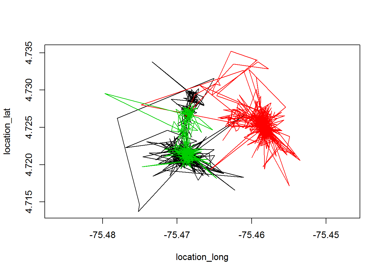
Basic plot
A basic plot of the tapir data:
plot(tapir, type="l")
S4 objects can be tricky to work with … for analysis R is much better suited to working with data frames and lists.
tapir.df <- as.data.frame(tapir)
str(tapir.df)
## 'data.frame': 5379 obs. of 12 variables:
## $ gps_dop : num 2.1 2.9 3.1 7 4.8 2.4 2.1 2.4 1.6 3.6 ...
## $ gps_time_to_fix : num 1 53 55 89 55 89 67 79 70 53 ...
## $ height_above_msl: num 1620 0 0 0 0 ...
## $ location_lat : num 4.73 4.73 4.73 4.71 4.71 ...
## $ location_long : num -75.5 -75.5 -75.5 -75.5 -75.5 ...
## $ timestamp : POSIXct, format: "2007-03-20 02:07:00" "2007-03-20 03:00:00" ...
## $ update_ts : Factor w/ 3 levels "2017-07-13 23:57:05.411",..: 1 1 1 1 1 1 1 1 1 1 ...
## $ sensor_type_id : int 653 653 653 653 653 653 653 653 653 653 ...
## $ deployment_id : int 303120166 303120166 303120166 303120166 303120166 303120166 303120166 303120166 303120166 303120166 ...
## $ event_id : num 3.4e+09 3.4e+09 3.4e+09 3.4e+09 3.4e+09 ...
## $ location_long.1 : num -75.5 -75.5 -75.5 -75.5 -75.5 ...
## $ location_lat.1 : num 4.73 4.73 4.73 4.71 4.71 ...GGmap
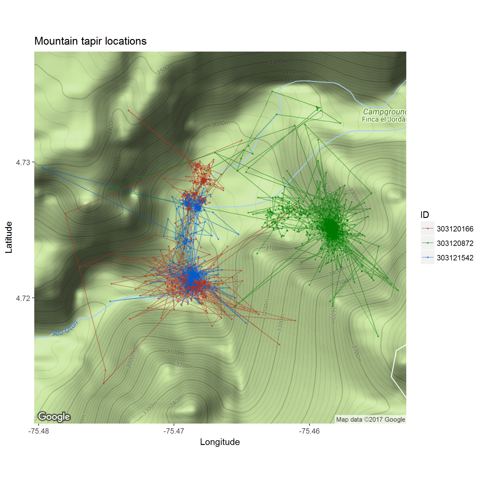
Here’s a quick ggmap of the tapirs:
require(ggmap)Generate “basemap” using the bounding boxes of the data.
basemap <- get_map(location = tapir@bbox, maptype = "terrain")To make the plot look better, we need to convert the deployment_id to a factor:
tapir.df$ID <- as.factor(tapir.df$deployment_id)Plot all the individuals:
ggmap(basemap) +
geom_path(data = tapir.df, mapping = aes(x = location_long, y = location_lat, col = ID), alpha = 0.5) +
geom_point(data = tapir.df, mapping = aes(x = location_long, y = location_lat, col=ID), alpha = 0.5, size=0.5) +
coord_map() + scale_colour_hue(l = 40) +
labs(x = "Longitude", y = "Latitude") + ggtitle("Mountain tapir locations") 
There are a few bells-and-whistles in this code to make it “prettier” that aren’t so important. But basically, you can see all the data at a glance, including some possible erroneous locations.
Practice
Download data from Movebank for an elk or a wolf of the Ya Ha Tinda study using R.