Annotating data with Movebank and R: Elevation and NDVI
Elie and Silvia
2017-08-09
To “Annotate” movement data means, simply, to match to location and time of an observation with some ancillary data, typically environmental data. There are many layers or observations and models, both static and dynamic, many obtained by remote sensing or weather modeling, that are available from a variety of sources. Here, we briefly describe how to use Movebank to annotate data, and then describe a few tools that allow for accessing elevation and MODIS data in R.
First, as always, lets load some of our favorite packages for data manipulation and visualization:
pcks <- c("plyr", "ggplot2", "ggmap", "ggthemes", "magrittr", "lubridate", "scales")
a <- lapply(pcks, require, character.only = TRUE, quietly = TRUE)
Annotating data with Movebank
Movebank includes an Env-Data tool for annotation. You can find a list of global environmental datasets available here. Highlights include: Topography and Bathymetry, MODIS land and ocean productivity, Derived topography variables such as slope, aspect and ruggedness, Wind variables and more (and expanding). Each of these comes with its own temporal and spatial resolution, which is matched as well as possible to the movement data.
To perform annotation: 1. go to the study site (e.g. the Tapir) and select Env-Data > Start Annotation Request. 2. Select the animals or tags you want to annotate. 3. Choose variables to request by name or type of variable and click on Continue. NB: for raster data, you will need to also select the type of interpolation you want (nearest-neighbor, bilinear, inverse-distance-weighted). 4. Review summary information on the data and click on Send annotation request. 5. Once the data is ready, you can download it as a csv table and plot in R.
Following the steps above for the Mountain Tapir data, are requesting the ASTER.ASTGTM2.Elevation digital elevation model, we can see at least one our tapirs moved up and down the mountain side, over about 250 m of elevation (thereby earning its name).
The downloaded and annotated data:
tapir1.annotated <- read.csv("_data/Tapir_GDEM.csv") %>%
    mutate(lon=location.long, lat=location.lat, GDEM = ASTER.ASTGTM2.Elevation)
str(tapir1.annotated)
## 'data.frame': 636 obs. of 17 variables:
## $ event.id : num 3.4e+09 3.4e+09 3.4e+09 3.4e+09 3.4e+09 ...
## $ visible : Factor w/ 1 level "true": 1 1 1 1 1 1 1 1 1 1 ...
## $ timestamp : Factor w/ 636 levels "2006-09-13 03:29:00.000",..: 1 2 3 4 5 6 7 8 9 10 ...
## $ location.long : num -75.5 -75.5 -75.5 -75.5 -75.5 ...
## $ location.lat : num 4.73 4.73 4.73 4.73 4.72 ...
## $ gps.dop : num 1.4 3.3 5.1 9.1 2.2 8 4.7 5 2.9 4.7 ...
## $ gps.time.to.fix : num 1 33 54 56 73 80 53 76 64 55 ...
## $ height.above.msl : num 2943 2943 0 0 0 ...
## $ sensor.type : Factor w/ 1 level "gps": 1 1 1 1 1 1 1 1 1 1 ...
## $ individual.taxon.canonical.name: Factor w/ 1 level "Tapirus pinchaque": 1 1 1 1 1 1 1 1 1 1 ...
## $ tag.local.identifier : Factor w/ 1 level "3(5TH-1360)-Tag": 1 1 1 1 1 1 1 1 1 1 ...
## $ individual.local.identifier : Factor w/ 1 level "3(5TH-1360)": 1 1 1 1 1 1 1 1 1 1 ...
## $ study.name : Factor w/ 1 level "Mountain tapir, Colombia": 1 1 1 1 1 1 1 1 1 1 ...
## $ ASTER.ASTGTM2.Elevation : num 2931 2911 2904 2915 2831 ...
## $ lon : num -75.5 -75.5 -75.5 -75.5 -75.5 ...
## $ lat : num 4.73 4.73 4.73 4.73 4.72 ...
## $ GDEM : num 2931 2911 2904 2915 2831 ...We’ve removed some outliers (following the code from the previous lesson) and saved a tidy file:
load("./_data/TapirAnnotatedAndCleaned.robj")
ggplot(tapir1, aes(x = lon, y = lat, color=GDEM)) + geom_path() + geom_point() + coord_fixed()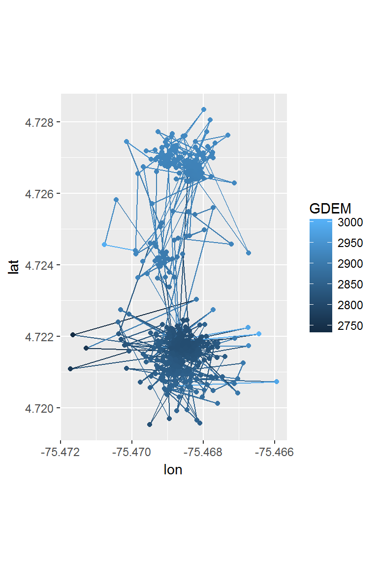
Annotating data in R
For a single study or a few individual, downloading .csv’s from Movebank is a reasonable strategy. But if you have a large study, it is nice to automate some of those steps as much as possible, and R provides a few useful tools. We will return, again, to our “cleaned up” moose data from the previous lesson:
load(file = "./_data/moose.df.rda")
head(moose.df)
## id nickname day.date time lon lat
## 1 179222573 M1 2009-03-08 2009-03-08 12:02:49 -119.9956 54.61333
## 2 179222573 M1 2009-03-09 2009-03-09 12:02:54 -120.0034 54.61424
## 3 179222573 M1 2009-03-10 2009-03-10 12:02:47 -120.0075 54.61564
## 4 179222573 M1 2009-03-11 2009-03-11 12:02:48 -120.0097 54.61492
## 5 179222573 M1 2009-03-12 2009-03-12 12:02:52 -120.0077 54.61534
## 6 179222573 M1 2009-03-13 2009-03-13 12:02:52 -120.0059 54.61548
## temp x y
## 1 -11.740833 306.5680 6055.888
## 2 -15.585833 306.0646 6056.011
## 3 -13.755833 305.8077 6056.178
## 4 -5.507500 305.6645 6056.104
## 5 3.464167 305.7941 6056.146
## 6 6.460000 305.9096 6056.156ggplot(moose.df, aes(x,y,color = nickname)) + geom_path() + coord_fixed()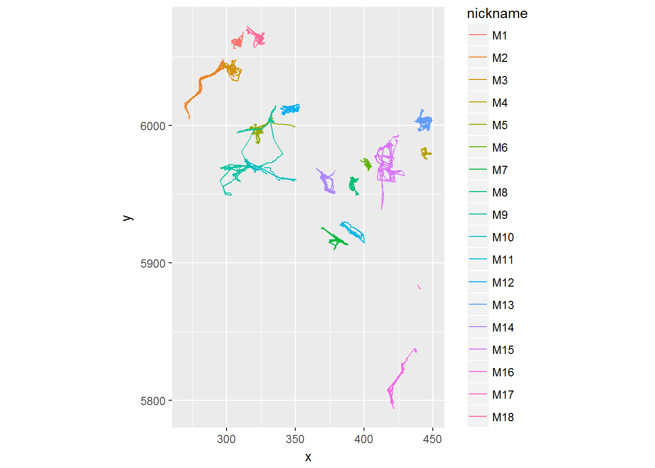
Elevations with elevatr
The elevatr package allows you to easily access the Mapzen terrain service. An example using one of the mooses:
require(elevatr)
me <- subset(moose.df, nickname == "M3")
proj <- "+proj=longlat +ellps=WGS84 +datum=WGS84 +no_defs"
m2 <- mutate(me, elevation = get_elev_point(data.frame(x = lon, y = lat), prj = proj, src = "mapzen", api_key = "mapzen-91tYY4s"))
m2$elevation <- as.numeric(m2$elevation@data[,1])
The function below modifies the scan.track function to let you visualize the migration in all three dimensions, and time.
scan.track.z <- function(time, x, y, z, title = "",...){
  par(mar = c(0,3,0,0), oma = c(4,4,2,2))
  layout(rbind(c(1,2), c(1,3), c(1,4)))

  MakeLetter <- function(a, where="topleft", cex=2)
     legend(where, pt.cex=0, bty="n", title=a, cex=cex, legend=NA)

  z.scaled <- (z - min(z))/(max(z) - min(z))

  plot(x,y,asp=1, type="o", pch=19, col=rgb(z.scaled,(1-z.scaled),0,.5), cex=0.5, ...); MakeLetter(title)
  plot(time,x, type="o", pch=19, col=rgb(0,0,0,.5), xaxt="n", xlab="", cex=0.5, ...); MakeLetter("X")
  plot(time,y, type="o", pch=19, col=rgb(0,0,0,.5), xaxt="n", xlab="", cex=0.5, ...); MakeLetter("Y")
  plot(time,z, type="o", pch=19, col=rgb(0,0,0,.5), cex=0.5, ...); MakeLetter("Z")
}
Illustrate:
with(m2, scan.track.z(time = time, x=x, y=y, z = elevation, title = "Moose 2"))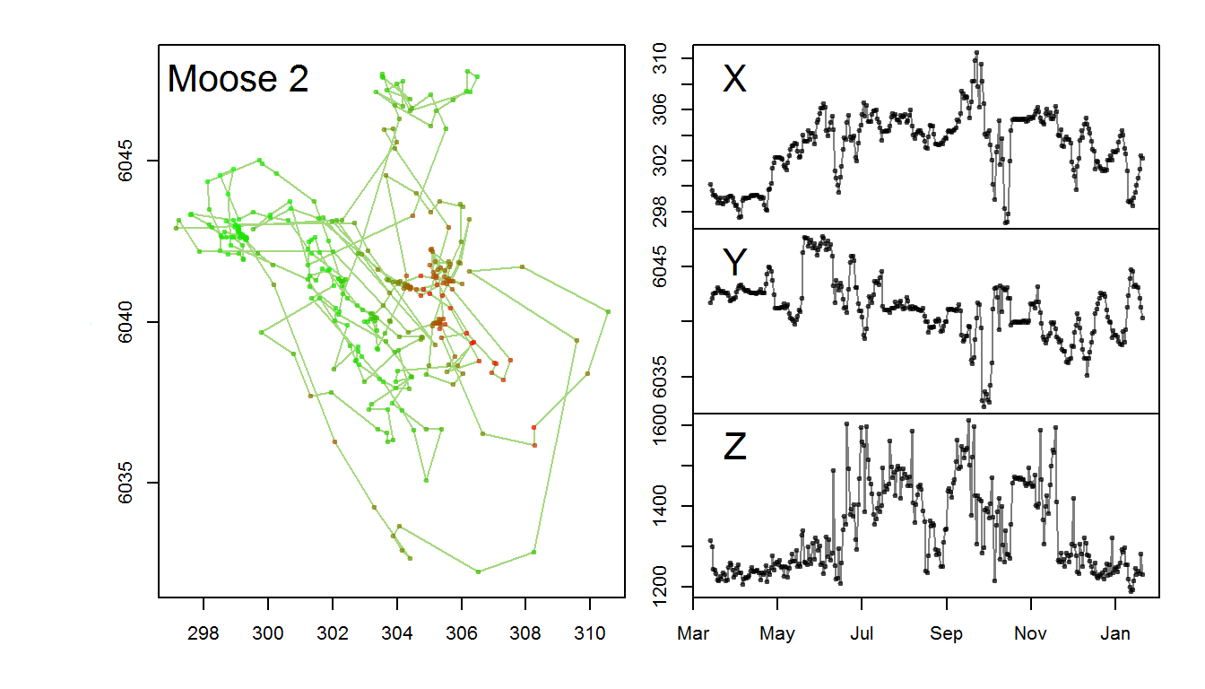
You can see here that in the summer months through November, the moose made multiple trips up and down the mountain side, but stayed mainly in low elevations in the winter through late spring.
Incidentally, lets see what the tapir is doing in time:
with(tapir1, scan.track.z(time = ymd_hms(timestamp), x=lon, y=lat, z = GDEM, title = "Mountain Tapir"))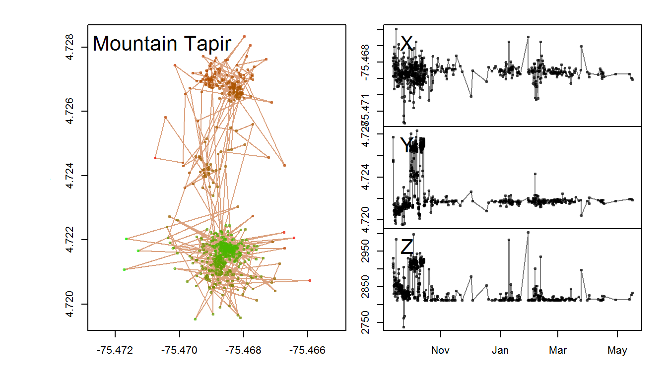
There’s no real winter/summer in Colombia, but this tapir, at least, seems to have mainly been interested in the higher elevations during a brief window in October.
NDVI with MODISTools
The R Package MODISTools provides: > “… an automated batch method for retrieving subsets of MODIS Land Processes data through the MODIS Web Service and processing them to a format ready for user friendly application in R such as statistical modelling.”
NB: A warning - when I tried this, the CRAN hosted version of MODISTools did NOT work because of outdated / unsupported dependencies (see this thread: https://groups.google.com/forum/#!topic/predicts_project/FctDowcYgx0), so you may have to install from GitHub as follows:
library(devtools)
install_git("http://github.com/seantuck12/MODISTools")
You may have to install a bunch of other dependent packages, (e.g. XML).
Once its installed, Load the package.
require(MODISTools)We’ll get the NDVI value for “MOD13Q1” at just two locations - one in the summer range and one at the winter range (note how close these are).
summer <- c(-119.7474, 53.84084)
winter <- c(-119.6198, 53.84184)
points <- rbind(summer, winter)

with(subset(moose.df, nickname == "M10"), plot(lon, lat, type="o", pch = 19, col=rgb(0,0,0,.5)))
points(points, col=2, pch = 4, cex=3, lwd=2)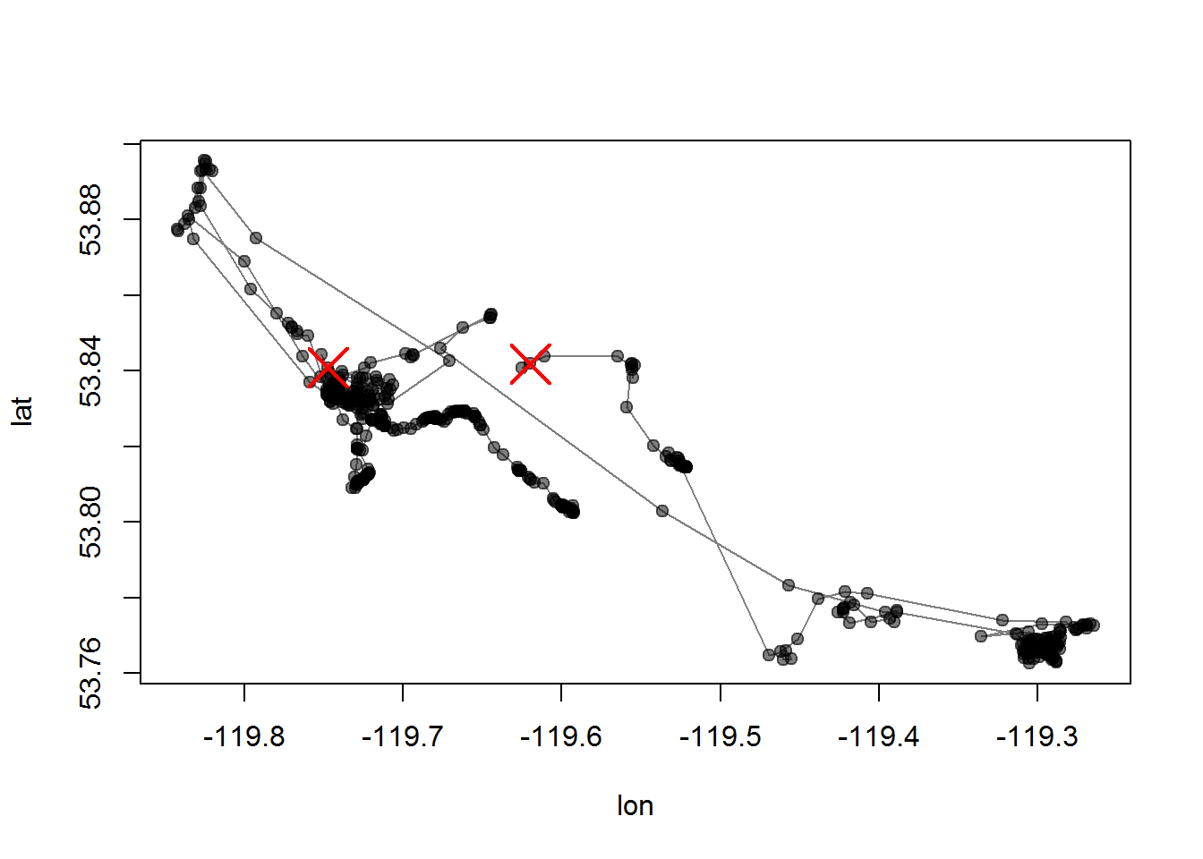
The available bands are:
product <- "MOD13Q1"
GetBands(product)
## [1] "250m_16_days_blue_reflectance"
## [2] "250m_16_days_MIR_reflectance"
## [3] "250m_16_days_NIR_reflectance"
## [4] "250m_16_days_pixel_reliability"
## [5] "250m_16_days_red_reflectance"
## [6] "250m_16_days_relative_azimuth_angle"
## [7] "250m_16_days_sun_zenith_angle"
## [8] "250m_16_days_view_zenith_angle"
## [9] "250m_16_days_VI_Quality"
## [10] "250m_16_days_NDVI"
## [11] "250m_16_days_EVI"
## [12] "250m_16_days_composite_day_of_the_year"Let’s go with NDVI
band <- c("250m_16_days_NDVI")
pixel <- c(0,0)
You have to specify the x/y/time range of the desired data:
period <- data.frame(lat=points[,2], long=points[,1], start.date=2008, end.date=2012, id=1)The key function (and this takes a while) is MODISSubsets. This will download a file and save it in the specified SaveDir. This takes a while … multiple minutes on my computer.
MODISSubsets(LoadDat = period, FileSep = "", Products = product, Bands = band, Size = pixel, SaveDir = "./_data", StartDate = TRUE)Files downloaded will be written to ./_data. Found 2 unique time-series to download. Getting subset for location 1 of 2... Getting subset for location 2 of 2... Full subset download complete. Writing the subset download file... Done! Check the subset download file for correct subset information and download messages.
This function downloaded two files: Lat66.65000Lon-152.00000Start2008-01-01End2012-12-31___MOD13Q1.asc and Lat67.30000Lon-150.75000Start2008-01-01End2012-12-31___MOD13Q1.asc.
These are difficult files to parse, but there are some functions that simplify their analysis. MODISTimeSeries extracts the time series from all the available .asc files in the directory as a matrix:
mooseNDVI.ts <- MODISTimeSeries(Dir = "./_data", Band = band, Simplify = TRUE)
head(mooseNDVI.ts)
## Lat53.84084Lon-119.7474Samp1Line1_pixel1
## A2008001 258
## A2008017 510
## A2008033 -119
## A2008049 183
## A2008065 -47
## A2008081 223
## Lat53.84184Lon-119.6198Samp1Line1_pixel1
## A2008001 1992
## A2008017 2844
## A2008033 1611
## A2008049 2459
## A2008065 3293
## A2008081 2291colnames(mooseNDVI.ts) <- c("ndvi.summer", "ndvi.winter")The row names of this matrix contain the date of the measurement, as the YEAR-DAYOFYEAR. This takes some manipulation to turn into a POSIX:
require(lubridate)
mooseNDVI.ts <- data.frame(mooseNDVI.ts, date = ymd(paste(substring(row.names(mooseNDVI.ts), 2,5), 1, 1)) +
  ddays(as.numeric(substring(row.names(mooseNDVI.ts), 6))))
Ok, now we can at least plot these NDVI bands underneath the migration of the moose:
with(mooseNDVI.ts,{
    plot(date, ndvi.summer, type="o", pch = 19, col = 2, ylab = "MODIS NDVI", ylim = c(-1000,9000))
    lines(date, ndvi.winter, type="o", pch = 19, col = 4)
})
legend("topleft", col = c(2,4), legend = c("summer range", "winter range"), pch = 19, lty = 1, cex=0.75)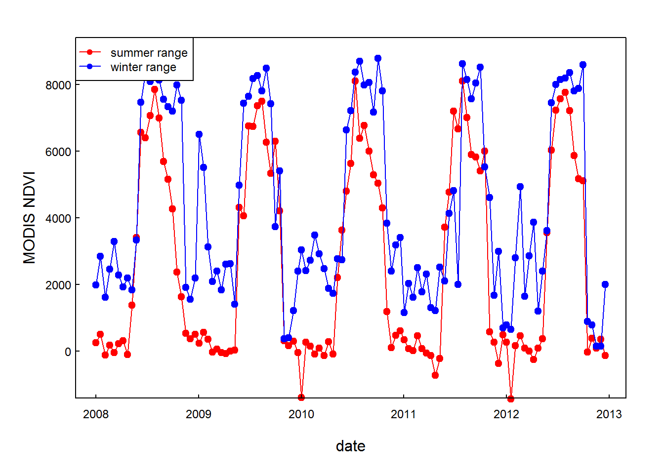
Although the winter range is very close to the summer range, it is a significantly better place to spend the winter - another nice preliminary observations.