Numerical Inference
BIOL709 / Winter 2018
Outline
- Review of inference and hypothesis testing
- Randomization and Permutation Tests
- The bootstrap
- Timing and profiling your code
The Question:
WHICH IS BIGGER?


Seed ant (Pogonomyrmex salinus) OR Thatch ant (Formica planipilis)
Step 1: load Data1
data.frame(subset(Ant[,c("Species","Weight","Headwidth1")], Species=="Seed"),
           subset(Ant[,c("Species","Weight","Headwidth1")], Species=="Thatch"))[1:15,]
## Species Weight Headwidth1 Species.1 Weight.1 Headwidth1.1
## 1 Seed 51 38 Thatch 90 39
## 2 Seed 55 41 Thatch 104 45
## 3 Seed 53 37 Thatch 106 40
## 4 Seed 48 35 Thatch 57 34
## 5 Seed 31 33 Thatch 90 43
## 6 Seed 72 39 Thatch 132 40
## 7 Seed 45 37 Thatch 91 42
## 8 Seed 65 40 Thatch 110 42
## 9 Seed 50 38 Thatch 86 41
## 10 Seed 102 43 Thatch 152 45
## 11 Seed 57 40 Thatch 74 38
## 12 Seed 38 39 Thatch 58 33
## 13 Seed 67 38 Thatch 71 33
## 14 Seed 57 37 Thatch 79 39
## 15 Seed 76 43 Thatch 67 35Step 2: Visualize Data
col<-c("turquoise","turquoise4","salmon","salmon4")
par(mfrow=c(1,2))
boxplot(Weight~Species,main="Weight (mg)",col=col[1:2], data=Ant)
boxplot(Headwidth1~Species,main="Head widths (mm)",col=col[3:4], data=Ant)
Step 3: Summary Statistics
Weight:
ddply(Ant, "Species", summarize, mean=mean(Weight), sd=sd(Weight))## Species mean sd
## 1 Seed 54.66667 13.98110
## 2 Thatch 92.80000 25.95806Head width:
ddply(Ant, "Species", summarize, mean=mean(Headwidth1), sd=sd(Headwidth1))## Species mean sd
## 1 Seed 38.5 2.270500
## 2 Thatch 39.7 3.495317The Question part 2:
- It certainly seems like Thatch ants might to be bigger than Seed ants.
- But there are obviously some Seed ants that are bigger than some Thatch ants!
- What does the question “Which is Bigger?” actually mean?
The short answer:
- It doesn’t mean anything stated simply… We need to refine the question!
The statement that A is bigger on average than B of the time is a start … But how do we know that this comparison isn’t an artifact of random sampling?
Again, there is no short answer. We need to rely on the framework of hypothesis testing - in which we assume a simpler version of reality, and see what the probability of our data is if the added structure (model) were not there.
Review of Hypothesis Testing.
- Since it can be tricky to even define what it is we want to know, we define it’s opposite, which is often simpler. This is the null hypothesis (\(H_0\)).
- What the null hypothesis isn’t we call the alternative hypothesis (\(H_1\) or \(H_A\)).
- We choose some summary of the data called the test statistic (\(\hat{\theta} \sim f(t)\)}).
- We create/compute/generate a null distibution of the test statistic… i.e.~the distribution we would expect of the test statistic if the null hypothesis were true.
- We calculate the observed value of the test statistic, \(\hat{\theta}^*\)}, and compare it to our distribution.
- We set some criterion - the critical region, within which we would fail to reject (not quite the same as ``accept’’) the null hypothesis. Here, two things can happen:
- If \(\hat{\theta}^*\) is ``extreme’’ (lies outside our critical region), we reject the null hypothesis}, accept the alternative hypothesis}, humbly acknowledging that we might be wrong, and call the probability that we might be wrong the Type I error.
- If \(\hat{\theta}^*\) is not ``extreme’’, we fail to reject the null hypothesis, calling the probability that we might be wrong the Type II error.
Randomization/ PTest
Step 1-2: Null and Alternative Hypotheses
 =
= 
\(H_0\): Seed and Thatch ants can be considered to come from the ``same’’ population. \
 <
< 
\(H_A\): Seed and Thatch ants come from different sized populations.
Step 3: Choose some test statistic
Something simple, like the difference between the means:
\[D_W = \overline{W_t} - \overline{W_s}\] \[D_H = \overline{H_t} - \overline{H_s}\]
Step 4: Null-distribution of the test statistic
- If the null hypothesis is true, then there is no difference between the two groups means we can resample them in any which way
- Randomization Test:
- shuffle all weights \(W\)
- split randomly into two new vectors: \(W_{S.sim}\)} and \(W_{T.sim}\)
- obtain and store the statistic $D_{W.sim} = - $
- Repeat steps 1-3 a bunch of times.
- Repeat for Heights
Randomization in R
Obtain observed statistic:
getD.means <- function(Y, X)   mean(Y[X==levels(X)[1]] - Y[X==levels(X)[2]])
(D.weight.obs <- with(Ant, getD.means(Weight, Species)))
## [1] -38.13333(D.head.obs <- with(Ant, getD.means(Headwidth2, Species)))## [1] -0.05046667Repeat many times, resampling the response (or the covariate) each time:
nreps <- 1000; D.weight.sim <- rep(0, nreps)
for(i in 1:nreps)
D.weight.sim[i] <- getD.means(Ant$Weight, sample(Ant$Species))
D.head.sim <- rep(0, nreps)
for(i in 1:nreps)
D.head.sim[i] <- getD.means(Ant$Headwidth2, sample(Ant$Species))
The above is the most basic template for a randomization test.
Visualize null-distribution and compute \(p\)-value
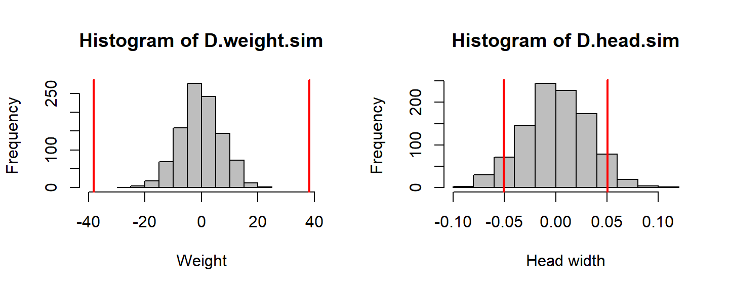
hist(D.weight.sim, col="grey", xlim=c(-40,40), xlab="Weight"); abline(v=c(-1,1)*D.weight.obs, col=2, lwd=2)
hist(D.head.sim, col="grey", xlab="Head width"); abline(v=c(-1,1)*D.head.obs, col=2, lwd=2)
Obtain randomization p-values \(= 2 \text{Pr}(\theta > |\widehat{\theta^*}|)\)
c(p.weight = 2*sum(D.weight.sim > abs(D.weight.obs))/nreps, p.height = 2*sum(D.head.sim > abs(D.head.obs))/nreps)## p.weight p.height
## 0.000 0.126What conclusions do we make based on these p-values?
R-Programming: Passing a function as a variable
Remember, you can pass a function into a function. This makes it very easy to perform randomization tests on ANY statistic. (Don’t forget the ellipsis: “…”)
  getD.fun <- function(Y, X, fun, ...)
    fun(Y[X==levels(X)[1]] - Y[X==levels(X)[2]], ...)

  getD.fun(Ant$Weight, Ant$Species, sd)
## [1] 27.14042 getD.fun(Ant$Weight, Ant$Species, quantile)## 0% 25% 50% 75% 100%
## -106.00 -55.25 -41.00 -17.75 9.00 getD.fun(Ant$Weight, Ant$Species, quantile, 0.75)## 75%
## -17.75R-Programming: the mosaic package and do()
The mosaic package - which is designed to provide some easy-to-use tools for randomization - makes naive loops more efficient with a funny little function called do():
require(mosaic)
do(5) * getD.fun(Ant$Weight, sample(Ant$Species), quantile)
## X0. X25. X50. X75. X100.
## 1 -71 -16.75 6.0 33.75 71
## 2 -66 -19.00 1.5 23.50 60
## 3 -73 -15.25 2.0 31.00 60
## 4 -95 -19.25 0.5 18.00 59
## 5 -45 -19.75 -3.5 21.50 81PRACTICE Using the functions above, test to see whether the variance of the Weights are significantly different between the two species of ant.
Randomization vs. Permutation
Note that every time we perform the operation above, we get a slightly different result and our test is therefore provides only an approximate \(p\)-value. With 30 of each kind of ant, it is prohibitive to try EVERY possible permutation (there are: \({60 \choose 30} = 1.18 \times 10^17\) possible ways to subsample these data for this test).
With much smaller samples we can compute an exact permutation test \(p\)-value.
Permutation test

Here are some data on mandible lengths of male and female jackals (Canis Aureus) from the British museum in London:
Y.m <- c(120, 107, 110, 116, 114, 111, 113)
Y.f <- c(110, 111, 107, 108, 110, 105)
There are 7 males and 6 females, so only 1716 ways to break up the data into those groups. The sample means are 113 and 108.5 mm, respectively, for males and females … so are males larger? Or, more precisely, what is the probability that \(D = 0\) given that \(D_{obs} = 4.5\)?
Code
require(gtools)  # For the combinations function

Z <- c(Y.m, Y.f)
C <- combinations(length(Z),length(Y.m))

getD.means <- function(index)
  mean(Z[index]) - mean(Z[-index])
Obtain observed statistics, and permutation distribution:
D.observed <- mean(Y.m) - mean(Y.f)
D.permuted <- apply(C, 1, getD.means)

sum(D.permuted > D.observed)/length(D.permuted)
## [1] 0.01282051sum(D.permuted >= D.observed)/length(D.permuted)## [1] 0.02447552Of ALL the possible combinations of 6 and 7 males and females, in only 22 was the null-male subset still larger than the observed difference of 4.5 mm.
[Note, that another 20 had a difference of EXACTLY 4.5! This frequently happens with small datasets].
Flashback: How did we do this before?
Without recourse to pretty rapid computation, statisticians had to pull all kinds of tricky and elegant contortions to obtain null distributions based not on *resampling} but on the central limit theorem and asymptotic results.
Recall that to compare two sample means, we used the \(T\) statistic: \[t^* = {\bar{X_1} - \bar{X_2} \over s_p \sqrt{ {1\over n_1} + {1\over n_2}}}\] where \[s_p^2 = {(n_1 - 1)s_1^2 + (n_2 - 1)s_2^2 \over n_1 + n_2 - 2},\] and that under the null hypothesis the statistic has a known distribution:
allowing us to compute \(p\)-values by merely looking up values of the cumulative probability in a table. Mathematically and manually - this is a much more complicated procedure, but computationally trivial (easy to do even by hand).
Some T-tests
t.test(Weight~Species, data=Ant)##
## Welch Two Sample t-test
##
## data: Weight by Species
## t = -7.0841, df = 44.519, p-value = 8.093e-09
## alternative hypothesis: true difference in means is not equal to 0
## 95 percent confidence interval:
## -48.97843 -27.28824
## sample estimates:
## mean in group Seed mean in group Thatch
## 54.66667 92.80000t.test(Headwidth2~Species, data=Ant)##
## Welch Two Sample t-test
##
## data: Headwidth2 by Species
## t = -1.5746, df = 49.754, p-value = 0.1217
## alternative hypothesis: true difference in means is not equal to 0
## 95 percent confidence interval:
## -0.11485025 0.01391691
## sample estimates:
## mean in group Seed mean in group Thatch
## 1.621033 1.671500How do these p-values compare to ours?
What did we have to assume to perform this text?
Some comments on classical inference
All of the so-called ``pivot-quantities’’ - \(z\)-scores, \(t\), Chi-squared and \(F\) statistics - all exploit the central limit theorem to fold up on themselves and reduce data to scale-free quantities with asymptotically known distributions with minimal free parameters. This contortion is very elegant (one Shakespeare versus a billion monkeys!), and a large amount of 20th century statistics was devoted to obtaining these quantities and understanding their properties and applicability. But their use comes with come constraints / assumptions:
    -  Residuals must be normally distributed,
-  A heavy reliance on the mean (and other moments) as measures of comparison between groups,
-  A strong assumption of independence in the sampling (can be relaxed ... but complciated),
-  An assumption of an observation arising from an infinite population.
Open Question: how much longer will we be teaching these tools as a core component of statistics? Are they the equivalent of Newton’s Mechanics 101 or Daguerrotyping 101?
Some comments on resampling inference
Computational statistics allows for relaxations of all (or most) of these constraints in different ways to different extents. In particular: permutation tests exist for any statistic, regardless of whether its distribution is known. There is absolute freedom in choosing a statistic which best discriminates between null and alternative hypotheses. Quick example: median of regional GDP:
GDP <- c(49683, 3163, 7983, 3228, 2962, 1950, 15741, 4171, 10373, 14621, 8866)
Region <- factor(c(rep("SEAsia", 6), rep("SAmerica", 5)))
tapply(GDP, Region, function(x) c(mean(x), median(x)))
## $SAmerica
## [1] 10754.4 10373.0
##
## $SEAsia
## [1] 11494.83 3195.50T-test of means:
t.test(GDP~Region)$p.value## [1] 0.9290917Permutation test of medians:
C <- combinations(length(GDP),table(Region)[1])
getD.median <- function(index, Y)
  median(Y[index]) - median(Y[-index])
D.observed <- diff(tapply(GDP, Region, median))
D.permuted <- apply(C, 1, getD.median, Y=GDP)
sum(D.permuted >= abs(D.observed)) / length(D.permuted)
## [1] 0.08008658R tool: lmPerm
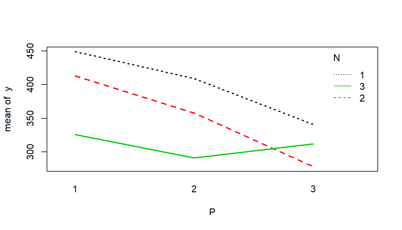
A package called lmPerm boasts the use of permutation tests to do anything lm() does. Let’s see how it works. Consider the following data on lettuce growth as a function of nitrogen (N) and potash (P) treatments:
require(lmPerm)
data(CC164)
CC164
## y P N Block
## 1 449 1 1 0
## 2 413 1 2 2
## 3 326 1 3 1
## 4 409 2 1 1
## 5 358 2 2 0
## 6 291 2 3 2
## 7 341 3 1 2
## 8 278 3 2 1
## 9 312 3 3 0Interaction plot:
with(CC164, interaction.plot(P,N,y, col=1:3, lwd=2))
Warning: This can happen to you: obsolete R package}
lmPerm was recently updated, but last year, I found it was no longer supported on CRAN … what to do?
You can install archived versions as follows:
url <- "https://cran.r-project.org/src/contrib/Archive/lmPerm/lmPerm_1.1-2.tar.gz"
download.file(url = url, destfile = pkgFile)
pkgFile <- "lmPerm_1.1-2.tar.gz"
install.packages(pkgs=pkgFile, type="source", repos=NULL)
unlink(pkgFile)
Permutation multi-factor analysis}
lmp(y ~ P * N, data = CC164, perm = "Exact") %>% summary## [1] "Settings: unique SS "##
## Call:
## lmp(formula = y ~ P * N, data = CC164, perm = "Exact")
##
## Residuals:
## ALL 9 residuals are 0: no residual degrees of freedom!
##
## Coefficients:
## Estimate Pr(Exact)
## P.L -60.575 0.0786 .
## P.Q 0.408 1.0000
## N.L -63.640 0.0643 .
## N.Q 4.082 0.8929
## P.L:N.L 47.000 0.4656
## P.Q:N.L 24.249 0.7075
## P.L:N.Q 42.724 0.5052
## P.Q:N.Q 13.000 0.8524
## ---
## Signif. codes: 0 '***' 0.001 '**' 0.01 '*' 0.05 '.' 0.1 ' ' 1
##
## Residual standard error: NaN on 0 degrees of freedom
## Multiple R-Squared: 1, Adjusted R-squared: NaN
## F-statistic: NaN on 8 and 0 DF, p-value: NAThis is “Exact”, because it computes all the p-values for all 9!=362,880 permutations. With 9, this is pretty instant.
According to authors: “12 needs 3 minutes, while 14 is an overnighter. No wonder permutations are seldomly used!”
lmPerm p-values
Easy enough to obtain approximtae \(p\)-values, which are computed efficiently because of a stoppage rule, e.g. when standard deviation of p-value falls below some fraction of the estimated p-value
summary(lmp(y ~ P * N, data = CC164, perm="Prob"))## [1] "Settings: unique SS "##
## Call:
## lmp(formula = y ~ P * N, data = CC164, perm = "Prob")
##
## Residuals:
## ALL 9 residuals are 0: no residual degrees of freedom!
##
## Coefficients:
## Estimate Iter Pr(Prob)
## P.L -60.5755 902 0.1009
## P.Q 0.4082 51 1.0000
## N.L -63.6396 2114 0.0454 *
## N.Q 4.0825 51 0.9412
## P.L:N.L 47.0000 173 0.3699
## P.Q:N.L 24.2487 58 0.6379
## P.L:N.Q 42.7239 102 0.5000
## P.Q:N.Q 13.0000 51 0.8627
## ---
## Signif. codes: 0 '***' 0.001 '**' 0.01 '*' 0.05 '.' 0.1 ' ' 1
##
## Residual standard error: NaN on 0 degrees of freedom
## Multiple R-Squared: 1, Adjusted R-squared: NaN
## F-statistic: NaN on 8 and 0 DF, p-value: NAAlso: ANOVA
anova(lmp(y ~ P * N, data = CC164, perm="Prob"))## [1] "Settings: unique SS "
## Analysis of Variance Table
##
## Response: y
## Df R Sum Sq R Mean Sq Iter Pr(Prob)
## P 2 11008.7 5504.3 1576 0.1967
## N 2 12200.0 6100.0 1392 0.2141
## P:N 4 4791.3 1197.8 136 0.8529
## Residuals 0 0.0Also:
- P-values for saturated models
- Polynomial surfaces
- Multiple responses
- Nice vignette!
BUT:
- You are limited to the typical regression type statistics (means, sums of squares, etc.)
Permutation final thoughts
So: if you can have complex data structure, multiple covariates, multiple responses, and you are interested in comparing means, but are (understandably) uncomfortable with the normality assumptions of ANOVA, are nervous about outliers, there is no reason not to use
lmPerm, which is (by definition) more robust to assumption violations thanlm(). As an added bonus if the number of rows in your data is small (or you have a megacomputer), you can always brag that your \(p\)-value is EXACT, and not dependent on some hundred-year-old asymptotics.
The Bootstrap

The idea is simple: Assume your sample represents the population, and that any time you resample from your sample, you are effectively sampling from the population, and the distribution of any statistic that you observe by resampling from your own sample reflects the distribution of that statistic in the population. \
Because you are relying only on your own data - (without any of the heavy-handed innovation-killing tax-happy bureaucracy of asymptotics) - it is as if you are raising yourself up by your bootstraps (or pony-tail).

Earthquake Data
Simplest example: Confidence intervals. Let’s find a highly non-normal data set (our old - yet ever renewing friend - the earthquakes of the world):
EQ <- read.csv("./data/earthquakes_20170105.csv")
# EQ <- read.csv("http://earthquake.usgs.gov/earthquakes/feed/v1.0/summary/all_month.csv")
And convert the times to POSIX.lt object:
EQ$time <- as.POSIXlt(EQ$time, format = "%Y-%m-%dT%H:%M:%S")
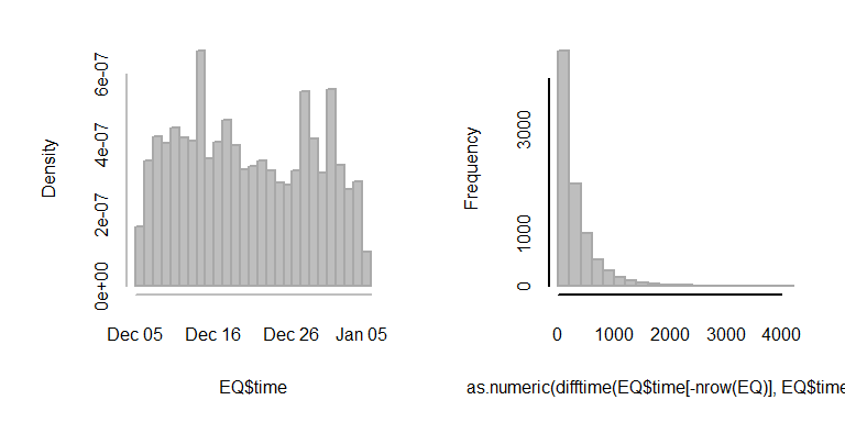
hist(EQ$time, col="grey", bor = "darkgrey", breaks=20, main="")
hist(as.numeric(difftime(EQ$time[-nrow(EQ)], EQ$time[-1])), col="grey", bor = "darkgrey", , breaks=20, main="")
Classical Confidence Intervals
Let’s pick out only earthquakes with magnitude > 6:
BigEQ <- subset(EQ, mag>=6)
dT.BigEQ <- as.numeric(na.omit(difftime(BigEQ$time[-nrow(BigEQ)], BigEQ$time[-1], units="min")))
sort(dT.BigEQ)
## [1] 36.43333 169.00000 223.11667 240.65000 257.35000 1098.78333
## [7] 1195.76667 1274.00000 1274.48333 1958.48333 2331.28333 2446.21667
## [13] 4849.83333 4896.76667 5203.73333 6247.86667 6605.20000And obtain the pivoted 95% Confidence Interval around the mean: \[ \widehat{\mu} = \overline{X} \pm t_{0.975, n-1} {s_x \over \sqrt{n}} \]
n <- length(dT.BigEQ)
mean(dT.BigEQ) + c(0,-1,1)*qt(0.975, df=n-1)*sd(dT.BigEQ)/sqrt(n)
## [1] 2371.116 1200.020 3542.212Or just:
t.test(dT.BigEQ)$conf.int## [1] 1200.020 3542.212
## attr(,"conf.level")
## [1] 0.95The interval is wide, because the data are highly variable and there are not so many points in the sample.
The Bootstrapped Confidence Intervals
Bootstrapped confidence interval, by hand:
nreps <- 1000; mean.BS <- rep(0,nreps)
for(i in 1:nreps)  mean.BS[i] <- mean(sample(dT.BigEQ, replace=TRUE))
quantile(mean.BS, c(0.025, 0.975))
## 2.5% 97.5%
## 1462.755 3405.446OR, with mosaic::do():
mean.BS <- do(nreps) * mean(sample(dT.BigEQ, replace=TRUE))
quantile(mean.BS[,1], c(0.025, 0.975))
## 2.5% 97.5%
## 1329.553 3470.795Just as easy to do for the median (of course):
median.BS <- do(nreps) * median(sample(dT.BigEQ, replace=TRUE))
quantile(median.BS[,1], c(0.025, 0.5, 0.975))
## 2.5% 50% 97.5%
## 257.350 1274.483 4849.833Note how the 97.5% quantile compares with the mean!
The boot package
This provides the boot() function, which acquires the bootstrapped distribution of any statistic applied to any data or model object. Here, we obtain a bootstrap on the correlation between magnitude and depth of earthquakes:
require(boot)
cor(BigEQ$mag, BigEQ$depth,  use= "complete.obs")
## [1] -0.1386588It is negative. But is it significantly negative? The correlation coefficient, even under null-assumptions of normality, does not have a trivial distribution2. But the bootstrapped version is quick and easy to obtain:
cor.bs <- boot(BigEQ,
function(x, i)
  cor(x$mag[i], x$depth[i], use= "complete"),
R = 1000)
(CI <- quantile(cor.bs$t, c(0.025, 0.975)))
## 2.5% 97.5%
## -0.3340204 0.2892403 hist(cor.bs$t, col="grey", main="")
abline(v = CI, col=2, lwd=2)
At least for large earthquakes in the last month (by mid-afternoon on May 7), deeper earthquakes have not been weaker than shallower earthquakes.
Practice: - Adapt this code to obtain a bootstrapped confidence interval around the regression slope of Magnitude against Depth.
Bootstrapped Prediction Intervals: on a glm
Using the example with the Portuguese sole posted here: http://faculty.washington.edu/eliezg/StatR201/VisualizingPredictions.html
Loading the data and fitting a binomial glm:
Solea <- read.csv("./data/Solea.csv")
Y <- Solea$Solea_solea
X <- Solea$salinity
Sole.glm <- glm(Y ~ X, family = "binomial")
expit <- function(x) exp(x)/(1 + exp(x))
Sole.predict <- predict(Sole.glm, newdata = data.frame(X = 0:40), se.fit = TRUE)
Parametric prediction intervals
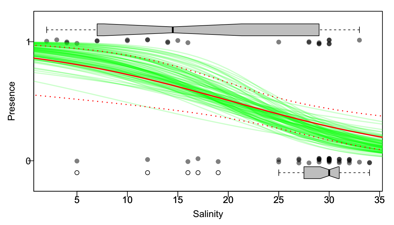
plot(X, jitter(Y, factor = 0.1), col = rgb(0, 0, 0, 0.5), pch = 19, ylim = c(-0.2,
    1.2), xlab = "Salinity", ylab = "Presence", yaxt = "n")
boxplot(X ~ Y, horizontal = TRUE, notch = TRUE, add = TRUE, at = c(-0.1, 1.1),
    width = c(0.1, 0.1), col = "grey", boxwex = 0.1, yaxt = "n")
axis(2, at = 0:1, las = 1)
lines(0:40, expit(Sole.predict$fit), col = 2, lwd = 2)
lines(0:40, expit(Sole.predict$fit + 2 * Sole.predict$se), col = 2, lty = 3, lwd=2)
lines(0:40, expit(Sole.predict$fit - 2 * Sole.predict$se), col = 2, lty = 3, lwd=2)
abline(h = c(0, 1), col = "grey", lty = 3)
Bootstrapped Prediction Intervals
Sole.bs <- data.frame(X,Y)
for(i in 1:100){
  Sole.glm.bs <- glm(Y ~ X, data = Sole.bs[sample(1:nrow(Sole.bs), replace=TRUE),],
                     family = "binomial")
  Sole.predict.bs <- predict(Sole.glm.bs, newdata = data.frame(X = 0:40), se.fit = TRUE)
  lines(0:40, expit(Sole.predict.bs$fit), col = rgb(0,1,0,.2), lwd = 2)
}
Exercise (to think about): How would you obtain a 95% bootstrapped envelope around those prediction intervals?
R Programming: benchmarking
Now that we are in randomization / resampling territory, it is becoming impossible to avoid loops (whether overt or hidden) - which multiply little inefficiencies many times over. It becomes worth our while to try to figure out how to speed some operations up. Compare five versions of getD.mean:
getD.meanA <- function(Y, X) mean(subset(Y, X==unique(X)[2])) - mean(subset(Y, X==unique(X)[1]))
getD.meanB <- function(Y, X) as.numeric(diff(tapply(Y,X,mean)))
getD.meanC <- function(Y, X) mean(Y[X==levels(X)[2]]) - mean(Y[X==levels(X)[1]])
getD.meanD <- function(Y, X)
{ which1 = X==levels(X)[2];  base::sum(Y[which1])/sum(which1) - base::sum(Y[!which1])/sum(!which1) }
getD.meanE <- function(Y, X){ daply(data.frame(Y,X), "X", summarize, mean(Y)) %>% unlist %>% diff}
R Programming: benchmarking
require(microbenchmark)
microbenchmark(
  a <- getD.meanA(Ant$Weight, Ant$Species), b <- getD.meanB(Ant$Weight, Ant$Species),
  c <- getD.meanC(Ant$Weight, Ant$Species), d <- getD.meanD(Ant$Weight, Ant$Species),
  e <- getD.meanE(Ant$Weight, Ant$Species))
## Unit: microseconds
## expr min lq mean
## a <- getD.meanA(Ant$Weight, Ant$Species) 768.495 824.3045 1013.1903
## b <- getD.meanB(Ant$Weight, Ant$Species) 578.617 611.1185 774.6577
## c <- getD.meanC(Ant$Weight, Ant$Species) 563.648 587.5975 738.8160
## d <- getD.meanD(Ant$Weight, Ant$Species) 371.632 391.0905 524.0823
## e <- getD.meanE(Ant$Weight, Ant$Species) 5848.171 6227.2870 8530.5894
## median uq max neval cld
## 865.5725 1010.1200 5674.544 100 a
## 639.5575 744.1185 3916.457 100 a
## 612.8290 675.9080 4998.423 100 a
## 408.4105 457.8045 7576.322 100 a
## 6899.1310 7938.1175 92236.025 100 bWhy is version D fastest? …. Why is version E so crazy slow?
Important check: Are the results identical?
identical(a,b,c,d,e)## [1] TRUELab 6/7 topics …
- benchmarking
- profiling
- big guns (like compiled code)
R Programming: Profiling your code
The Rprof() function allows for detailed profiling of the time it takes to perform certain tasks.
Rprof("Rprof.out")
a <- do(1000) * getD.meanB(Ant$Weight, Ant$Species)
Rprof(NULL)
This opens a connection to a file called: , writes a lot of information into it, which you can then summarize using:
summaryRprof("Rprof.out")Because the output is complex, we’re better off looking at “live” in R proper.
Comments on resampling inference
Resampling places just as much (or more!) emphasis on well-formulated hypotheses and awareness of assumptions when designing tests and making inference.
For example, can you design a permutation/randomization test that compares the means of two samples with unequal variance? It’s not easy!
In general, permutation/randomization-type tests test equality of distibutions: \(F_1 = F_2\), whereas BOOTSTRAP methods are better at testing parameters \(\theta_1 = \theta_2\). }