Lab 7: Basic Inference, Pivot Statistics and Tests

1. Inference

1.1. Point Estimate of Bernoulli Trial

Note: I lifted the following examples directly from The Cartoon Guide To Statistics, which is a great book for grasping some basic (but slippery) statistical concepts.

Suppose the Bernoulli Tack Factory is churning out brass tacks, some of which (inevitably) are defective. You want to know guess the the true proportion p of defective tacks is. So you sample n=1000 tacks, and, say, x = 832 are good ones. Obviously, our best guess for the probability is \(\widehat{p} = x/n = 832/1000 = 0.832\).

Now we ask: “How good is this estimate?” This is answered with a point estimate and a confidence interval (at a certain confidence level, e.g. 95%).

The basic way you makea 95% confidence interval here is:

1. find the point estimate (here: \(\widehat{p} = 0.832\))
1. determine the standard deviation of the estimate \(\sigma(\widehat{p}) = \sqrt{\frac{p(1-p)}{n}}\)
1. use the properties of the sampling distribution (usually: assuming normality) identify the range which captures the confidence level. At large sample sizes we can and assume that this random variable is normally distributed, and therefore 95% of the mass of this distribution is within 2 (or more precisely 1.96 [or even more precisely qnorm(0.975)]) standard deviations within the mean. Thus \(\widehat{p} \pm 1.96 \sigma(\widehat{p})\).

Ok, in R:

x <- 832
n <- 1000
p.hat <- x/n
z.critical <- qnorm(0.975)
p.hat.sd <- sqrt(p.hat*(1-p.hat)/n)
p.CI <- p.hat + c(-1,1)*z.critical*p.hat.sd
p.CI

## [1] 0.808828 0.855172

We can draw this estimate:

curve(dnorm(x, mean=p.hat, sd = p.hat.sd), xlim=c(0,1), col=2, n=1000, xlab="p.hat", ylab="density", bty="l")
abline(v = p.hat, lty=2)
abline(v = p.CI, lty=3)

This is a very narrow confidence interval, suggesting it is unlikely that the true probability of a good tack is less than 80%.

Exercise 1: Write a function (called getP) that returns a point estimate and confidence interval for a probability estimate at an arbitrary confidence level.

Try it out, assuming we sampled just 100 tacks, and counted 89 good ones.

getP(x = 89, n = 100, conf.level = 0.95)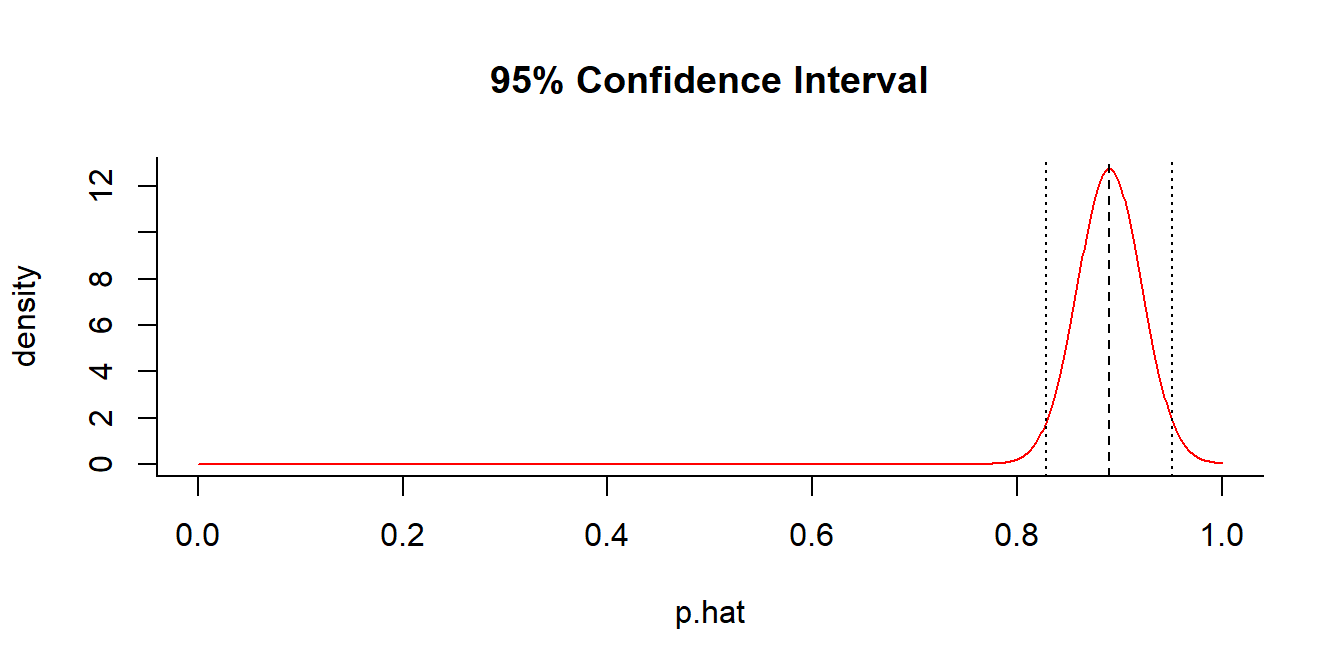

## $p.hat
## [1] 0.89
## 
## $p.CI
## [1] 0.8286747 0.9513253

What about at 99% confidence?

getP(x = 89, n = 100, conf.level = 0.99)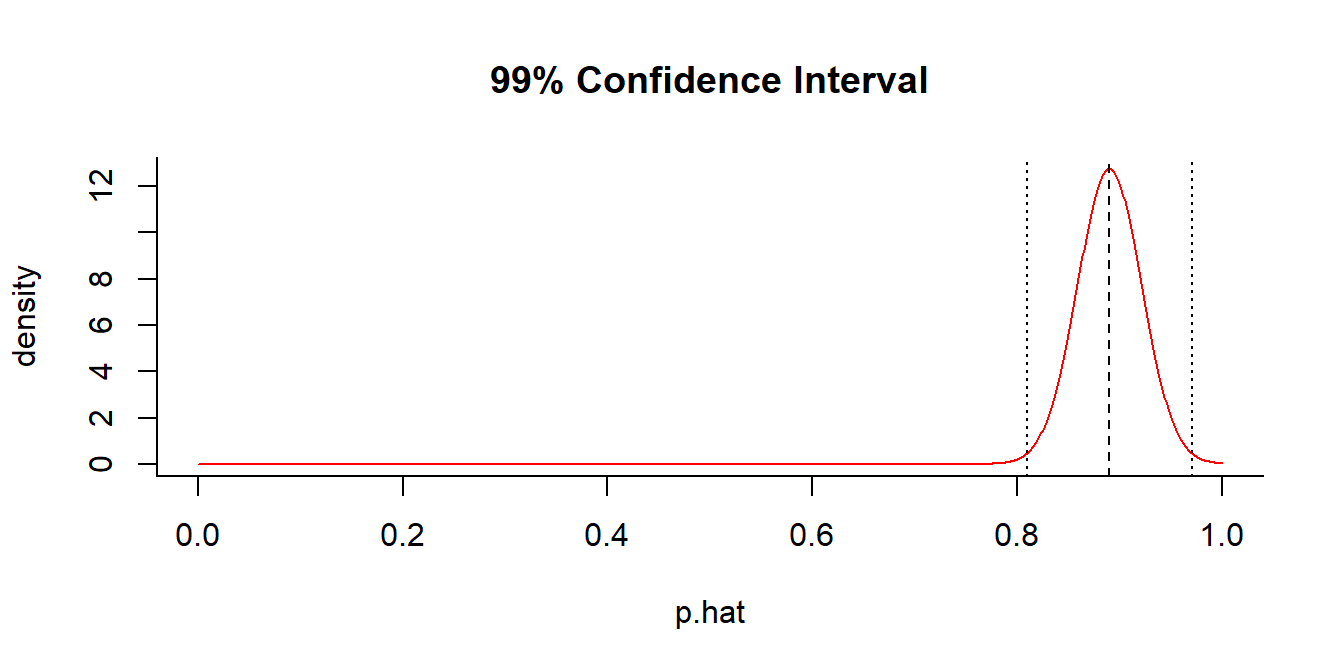

## $p.hat
## [1] 0.89
## 
## $p.CI
## [1] 0.8094049 0.9705951

1.2. Hypothesis Test for Bernoulli trial

Lets go back to the brother who suspects that spinning a coin is not `fair’, and therefore spins it 100 times and finds 60 tails. In the lecture, we talked about how setting up the confidence interval. We can use the code above:

getP(x = 60, n = 100, conf.level = 0.95)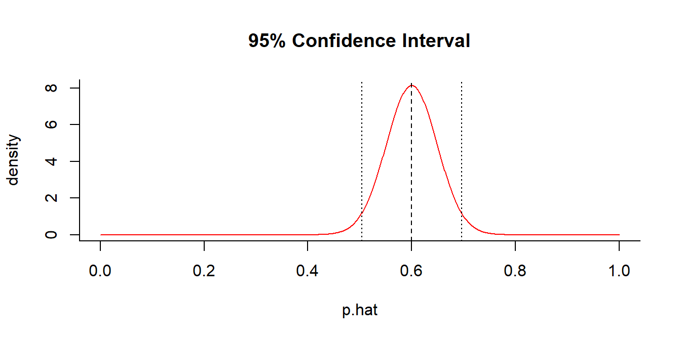

## $p.hat
## [1] 0.6
## 
## $p.CI
## [1] 0.5039818 0.6960182

A fair coin is just outside the 95% C.I.

This is also a very natural set-up for a hypothesis test of fairness. Recall the steps: 1. we specify \(H_0: p = 0.5\) 2. we specify \(H_a: p > 0.5\) 3. we assess the probability of such an extreme event.

Under the null-hypothesis, \(X \sim \text{Bernoulli}(n=100, p=0.5)\). So, the probability of getting a 60 or above is: \[ \sum_{i=60}^{100} f(x|n=100,p=0.5) \]

In R:

1 - pbinom(59, size=100, p=0.5)

## [1] 0.02844397

or:

sum(dbinom(60:100, size=100, p=0.5))

## [1] 0.02844397

This probability is smaller than the typical significance level of 0.05, so at that level we reject \(H_0\).

A simple test of proportions can be done in R with the following command:

prop.test(x=60, n=100, p=0.5)

## 
##  1-sample proportions test with continuity correction
## 
## data:  60 out of 100, null probability 0.5
## X-squared = 3.61, df = 1, p-value = 0.05743
## alternative hypothesis: true p is not equal to 0.5
## 95 percent confidence interval:
##  0.4970036 0.6952199
## sample estimates:
##   p 
## 0.6

This is the first bit of automatically generated statistical output we have seen in R. Note that according to this output, the p-value is 0.05743, which is typically not considered significant. Why is it different? Because the test was two-sided, i.e. we tested more rigorously “Is the Coin Fair?” versus “Is the Coin Biased Towards Tails?” In order to test the second test, we specify the alternative:

prop.test(x=60, n=100, p=0.5, alternative="greater")

## 
##  1-sample proportions test with continuity correction
## 
## data:  60 out of 100, null probability 0.5
## X-squared = 3.61, df = 1, p-value = 0.02872
## alternative hypothesis: true p is greater than 0.5
## 95 percent confidence interval:
##  0.5127842 1.0000000
## sample estimates:
##   p 
## 0.6

This result agrees almost exactly with our own p-value. The difference is that they use, essentially, the normal approximation.

1 - pnorm(59.5, mean=50, sd=sqrt(.5*.5*100))

## [1] 0.02871656

[In fact, R uses a slightly different and more general test statistic called the Chi-squared statistic, but for the case of a single proportion compared to a null proportion, the Chi-squared and normal approximation collapse to the same test.]

1.3. Point estimate of mean with known variance

Let’s quickly consider the dog problem. We randomly find 4 dogs of length (knowing, somehow, that the global s.d. for dogs is 20 cm):

Dog <- c(80,85,60,115)

How to construct a confidence interval?

n <- length(Dog)
Dog.mean <- mean(Dog)
Dog.sd <- 20
Dog.CI <- Dog.mean + qnorm(0.975) * c(-1,1) * Dog.sd/sqrt(n)
Dog.CI

## [1]  65.40036 104.59964

Exercise 2: Write a function that takes a sample X with known s.d. and returns its point estimate and confidence interval.

Example:

GetCI(Dog, sd=20)

## $estimate
## [1] 85
## 
## $CI
## [1]  65.40036 104.59964

GetCI(Dog, sd=20, conf.level=0.99)

## $estimate
## [1] 85
## 
## $CI
## [1]  59.24171 110.75829

Recall, that this result says that there is a 95% probability that the true mean lies somewhere within this interval. Let’s try to illustrate the way inference fundamentally inverts probability statements.

Create a vector of the entire dog population, draw a histogram, and illustrate our confidence interval using segments(x0,y0,x1,y1):

Dogs <- rnorm(100000, mean=100, sd=20)
hist(Dogs, col="grey", breaks=100, bor="grey")
abline(v=100, col=2, lwd=2)
myCI <- GetCI(Dog, sd=20, conf.level=0.95)$CI
segments(myCI[1], 0, myCI[2], 0, lwd=2)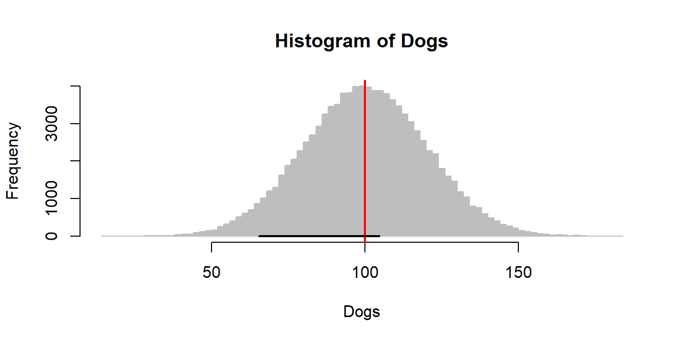

We are going to sample 4 dogs out of this population many many times, and plot their confidence interval on this histogram

hist(Dogs, col="grey", breaks=100, bor="grey")
abline(v=100, col=2, lwd=2)
c<-0
for(i in 1:1000)
{
  col <- 1
  myCI <-  GetCI(sample(Dogs,4), sd=20, conf.level=0.95)$CI
  # count the ones that don't surround the mean
  if(min(myCI) > 100 | max(myCI) < 100)
      {c <- c+1; col <- 3}
  if(i*30 < 4000)
  segments(myCI[1], i*30, myCI[2], i*30, lwd=2, col=col)
}

c/1000

## [1] 0.052

Notice, how approximately 5% of all the confidence intervals actually DO miss the true mean.

Exercise 3: Try performing this experiment with a highly non-normal distribution, for example your model of earthquake waiting times.

1.4. Hypothesis test of sample mean against known population

We sampled 25 Sri Lankan strays, and here is their data:

Dog.SL <- c(82, 109, 127, 124, 64, 88, 116, 83, 83, 99, 85, 127, 104, 85, 70, 88, 98, 81, 101, 104, 76, 92, 64, 59, 91)
mean(Dog.SL)

## [1] 92

We want to test the hypothesis (at 0.05 significance) that they are smaller than the reference population of global dogs (mean = 100 cm, s.d. = 20 cm).

Specify \(H_0: \mu = \mu_0\)
Specify \(H_a: \mu < \mu_0\)
Test statistic: \(z_{test} = \frac{\overline{X} - \mu_0}{\sigma/\sqrt{n}}\)
Distribution of test statistic under \(H_0\): \(Z \sim {\cal N}(0,1)\).
\(P\)-value: \(Pr(z_{test} < Z)\)

n <- length(Dog.SL)
X.bar <- mean(Dog.SL)
sigma <- 20
mu.0 <- 100
z.test <- (X.bar - mu.0)/(sigma/sqrt(n))
1-pnorm(abs(z.test))

## [1] 0.02275013

Quick exercise 4: How do we make this a two-sided test?

This is called the “Z-test”, and it is so basic it does not have an automatic little function in R. However, the following one-liner of code performs something very similar:

 t.test(Dog.SL, mu=100, alternative="less")

## 
##  One Sample t-test
## 
## data:  Dog.SL
## t = -2.1004, df = 24, p-value = 0.02319
## alternative hypothesis: true mean is less than 100
## 95 percent confidence interval:
##      -Inf 98.51634
## sample estimates:
## mean of x 
##        92

Why “T”? Why is the p-value a little greater? What does df stand for? These are topics for next week.

2. Chi-squared, F and T distributions

2.1 With respect to the normal distribution

Let’s illustrate each of these, all with respect to the normal distribution.

The Chi-squared distribution is a sum of n squared normal distributions. A single normal squared is:

Z <- rnorm(1000)
hist(Z^2, freq=FALSE, breaks=40, col="grey")
curve(dchisq(x, df = 1), add=TRUE, lwd=3, n=1000)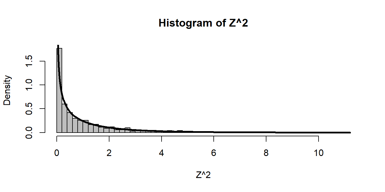

Three normals squared gives:

Z1 <- rnorm(1000)
Z2 <- rnorm(1000)
Z3 <- rnorm(1000)

hist(Z1^2 + Z2^2 + Z3^2, freq=FALSE, breaks=40, col="grey")
curve(dchisq(x, df = 3), add=TRUE, lwd=3, n=1000)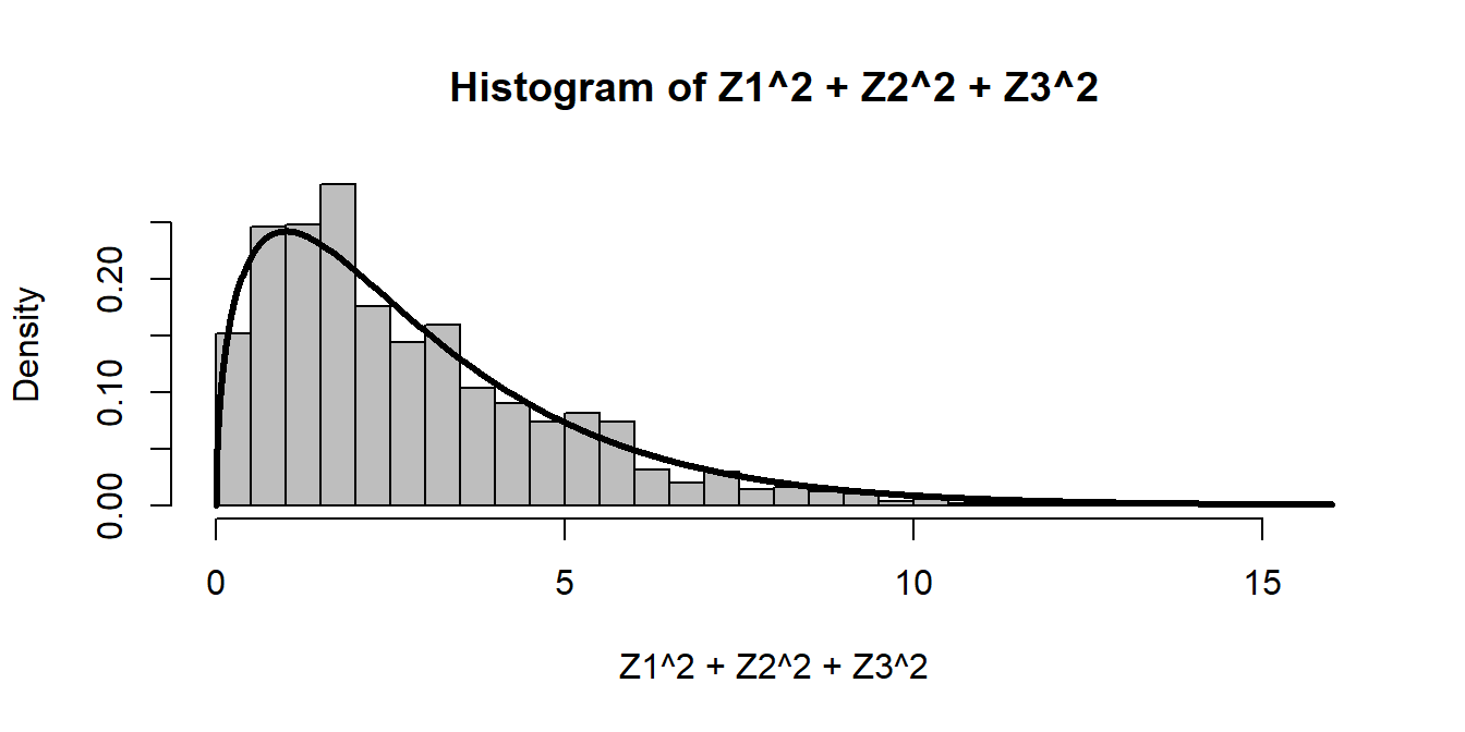

Note, we could generate this distribution without separately creating normals, and without a loop, by making an n x k matrix:

n <- 5
Z.matrix <- matrix(rnorm(n*1000), ncol=n)
X <- rowSums(Z.matrix^2)
hist(X, freq=FALSE, breaks=40, col="grey")
curve(dchisq(x, df = n), add=TRUE, lwd=3, n=1000)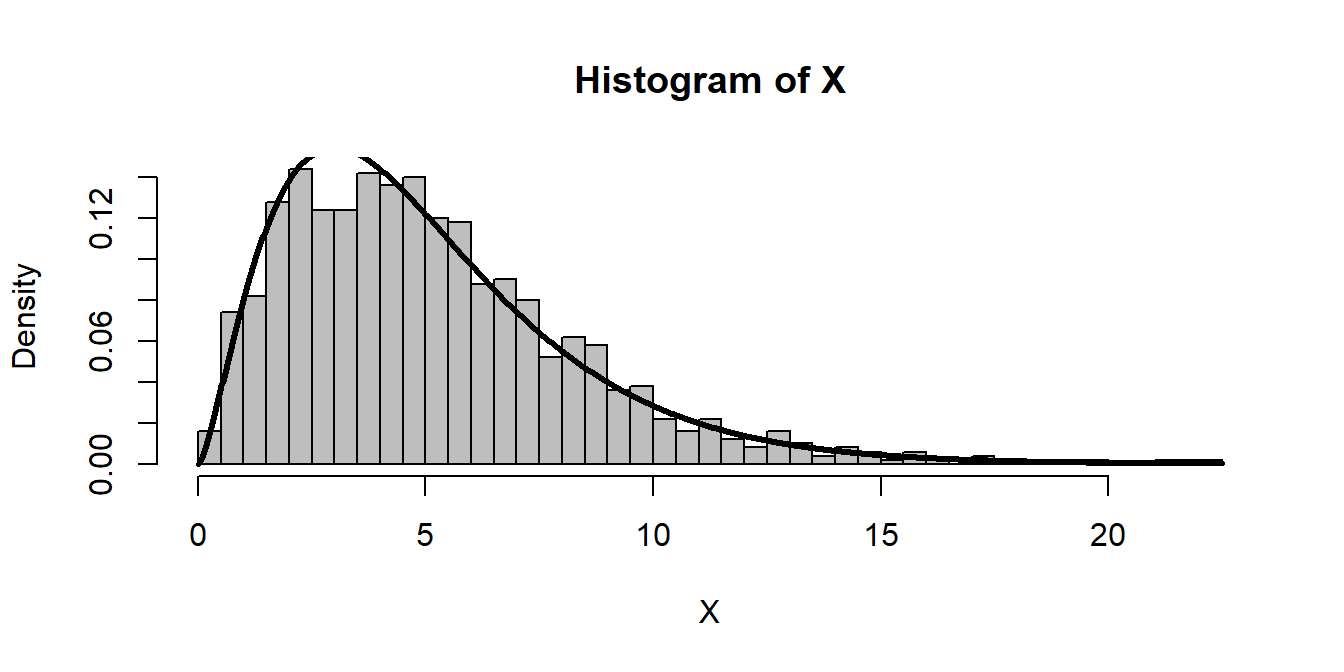

The T-distribution is given by the ratio of a standard normal and the square root of the chi-squared divided by its degrees of freedom. Thus:

df <- 4
Z <- rnorm(1000)
Y <- rchisq(1000, df)
T <- Z/sqrt(Y/df)
hist(T, freq=FALSE, breaks=50, col="grey", ylim=c(0,dt(0,df)*1.5), xlim=c(-15,15))
curve(dt(x, df = df), add=TRUE, lwd=3, n=1000)
curve(dnorm(x), add=TRUE, col="red", lty = 3, n=1000, xpd=TRUE)

The F-distribution is given by the ratio of chi-squared variables, divided by their degrees of freedom.

df1 <- 4
df2 <- 10

Y1 <- rchisq(1000, df1)
Y2 <- rchisq(1000, df2)

F <- (Y1/df1)/(Y2/df2)
hist(F, freq=FALSE, breaks=50, col="grey")
curve(df(x, df1 = df1, df2 = df2), add=TRUE, lwd=3, n=1000)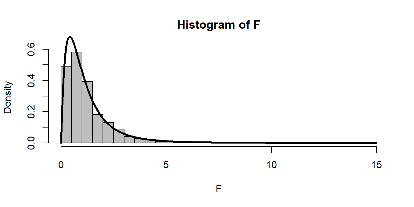

Note that in the presentation, I would sometimes have several plots laid out in a non a x b grid. This can be done in R with the layout() command, which takes a matrix of integers (1,2,3, …) and lays out figures according to the matrix.

Thus:

layout(rbind(c(1,2),c(3,3)))
layout.show(3)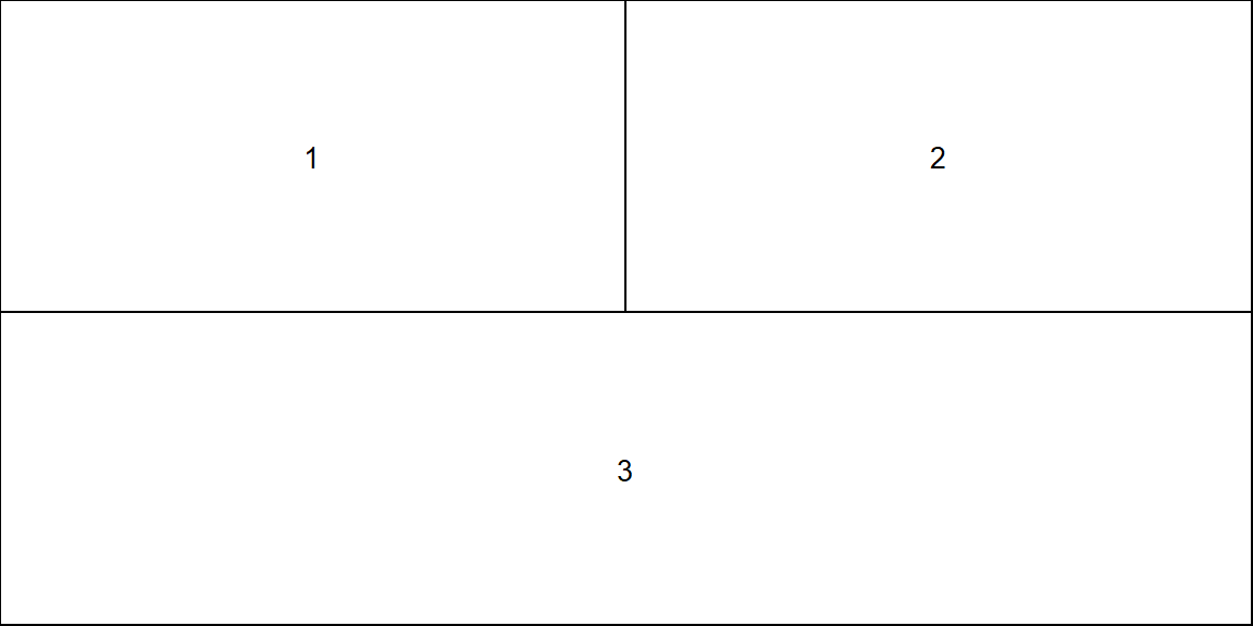

We can use this to illustrate multiple figures creatively:

layout(rbind(c(1,2),c(3,3),c(3,3)))
hist(Y1, freq=FALSE, breaks=50, col="orange"); curve(dchisq(x, df1), add=TRUE, lwd=3)
hist(Y2, freq=FALSE, breaks=50, col="purple"); curve(dchisq(x, df2), add=TRUE, lwd=3)
hist((Y1/df1)/(Y2/df2), freq=FALSE, breaks=50, col="blue"); curve(df(x, df1, df2), add=TRUE, lwd=3)

2.2 With respect to sampling distribution

Consider some population X with some distribution:

X <- -rgamma(100000, 3,1/2)
hist(X, col="grey")

mean(X)

## [1] -6.005343

var(X)

## [1] 12.06099

Here, we happen to know that the mean and variance are -6 and 12.

According to theory, if we sample some n from this distribution, then: \[ \frac{\overline{X} - \mu}{\sigma/\sqrt{n}} \sim {\cal N}(0,1)\\ (n-1)\frac{s^2}{\sigma^2} \sim {\chi^2}(\nu = n-1)\\ \frac{\overline{X} - \mu}{s/\sqrt{n}} \sim {\cal T}(\nu = n-1) \] and if we have two samples: \(X_1\) and \(X_2\) of size \(n_1\) and \(n_2\), then: \[ \frac{s_1^2}{s_2^2} \sim {\cal F}({\nu_1 = n_1-1, \nu_2 = n_2-1}) \] These are all straightforward to illustrate.

Exercise: Simulate three vectors X.bar, S1 and S2 that are the sample mean and sample standard drawn from X with sample sizes n = 10 n = 10 and n = 20 respectively, each repeated 1000 times.

Once you’ve obtained these vectors, it is straightforward to illustrate the theoretical predictions above:

layout(rbind(c(1,1), c(2,3),c(4,5)))
par(xpd=TRUE, cex.main=1.5)
hist(X, col="grey", freq=FALSE, breaks=40)

hist((X.bar - mu)/(sigma/sqrt(n1)), freq=FALSE,col=rgb(1,0,0,.2), bor=rgb(1,0,0,.6), main="Z")
curve(dnorm(x), add=TRUE, lwd=2, col="red")

hist((n1-1)*S1^2/sigma^2, freq=FALSE,col=rgb(0,1,0,.2), bor=rgb(0,1,0,.6), main="Chi-Squared")
curve(dchisq(x, df=n1-1), add=TRUE, lwd=2, col="darkgreen")

hist((X.bar - mu)/(S1/sqrt(n1)), freq=FALSE,col=rgb(0,0,1,.2), bor=rgb(0,0,1,.6), main="T")
curve(dnorm(x), add=TRUE, lwd=2, col="darkblue")

hist(S1^2/S2^2, freq=FALSE,col=rgb(0.5,0,0.5,.2), bor=rgb(0.5,0,0.5,.6), main="F", breaks=40)
curve(df(x, n1, n2), add=TRUE, lwd=2, col="purple")

3. Tests!

3.1 Single and Two-sample T-test

Let’s consider the 16 Sri Lankan strats dogs in the first t-test example:

Dogs <- c(69, 90, 91, 96, 97, 108, 54, 96, 114, 90, 102, 75, 85, 67, 112, 126)
(X.bar <- mean(Dogs))

## [1] 92

(s <- sd(Dogs))

## [1] 18.97015

The test statistic for the test against \(\mu = 100\) is:

n <- length(Dogs)
mu <- 100
t.obs <- (X.bar - mu)/(s/sqrt(n))
t.obs

## [1] -1.68686

p.value <- pt(t.obs, df=n-1)
p.value

## [1] 0.05615497

The p.value is not significant at the \(\alpha=0.05\) level. Note, all of this can be done with the simple command:

t.test(Dogs, mu=100, alternative="less")

## 
##  One Sample t-test
## 
## data:  Dogs
## t = -1.6869, df = 15, p-value = 0.05615
## alternative hypothesis: true mean is less than 100
## 95 percent confidence interval:
##      -Inf 100.3139
## sample estimates:
## mean of x 
##        92

Lets compare the two samples (the Sri Lankan and the thoroughbred dogs):

Dogs2 <- c(89, 91, 112, 124)
(mean(Dogs2))

## [1] 104

(sd(Dogs2))

## [1] 16.91153

t.test(Dogs, Dogs2)

## 
##  Welch Two Sample t-test
## 
## data:  Dogs and Dogs2
## t = -1.2378, df = 5.0837, p-value = 0.2699
## alternative hypothesis: true difference in means is not equal to 0
## 95 percent confidence interval:
##  -36.79875  12.79875
## sample estimates:
## mean of x mean of y 
##        92       104

3.2 Paired T-test

Load the taxi data:

Taxi <- 1:10
GasA <- c(27.01, 20, 23.41, 25.22, 30.11, 25.55, 22.23, 19.78, 33.45, 25.22)
GasB <- c(26.95, 20.44, 25.05, 26.32, 29.56, 26.6, 22.93, 20.23, 33.95, 26.01)
boxplot(GasA, GasB, col="grey")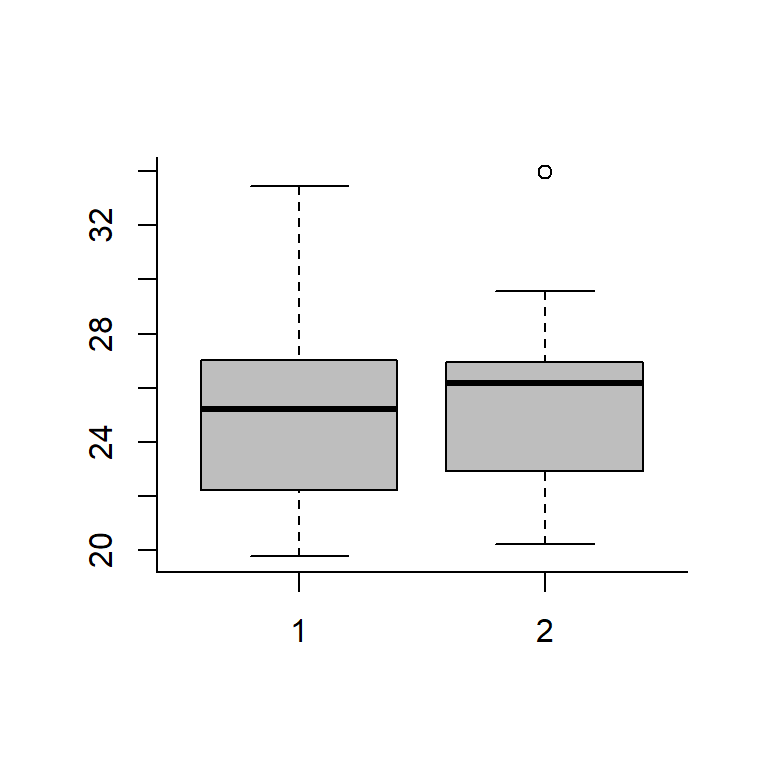

Compare using a straightforward t-test:

t.test(GasA, GasB)

## 
##  Welch Two Sample t-test
## 
## data:  GasA and GasB
## t = -0.32371, df = 17.971, p-value = 0.7499
## alternative hypothesis: true difference in means is not equal to 0
## 95 percent confidence interval:
##  -4.539425  3.327425
## sample estimates:
## mean of x mean of y 
##    25.198    25.804

Small t-statistic and high p-value - NOT a significant difference.

But if we perform the hypothesis on the difference:

D <- GasA - GasB
hist(D, col="grey")
abline(v=0, col=2, lty=3, lwd=3)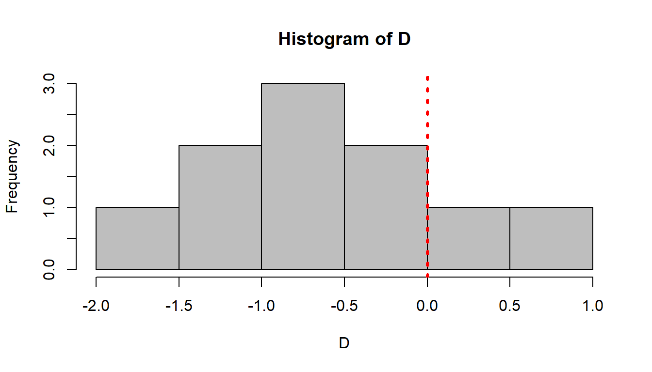

Just looking at the histogram, it looks like the difference may be negative. We test it via:

t.test(GasA, GasB, paired=TRUE)

## 
##  Paired t-test
## 
## data:  GasA and GasB
## t = -3.1197, df = 9, p-value = 0.01233
## alternative hypothesis: true difference in means is not equal to 0
## 95 percent confidence interval:
##  -1.0454282 -0.1665718
## sample estimates:
## mean of the differences 
##                  -0.606

Now, we see that there really is a significant differnce,

Quick Question: Is this different than testing whether the difference between the two is different than 0? Find out by doing a quick t-test on the difference.

3.3 F-test on variances

The NBA games example:

Year2010 <- c(100, 95, 97, 101, 100, 94, 110, 105, 98, 109)
Year2011 <- c(111, 108, 99, 94, 115, 100, 88, 75, 98, 90)
boxplot(Year2010, Year2011, col="yellow", bor="blue", ylab="Points Scored")
axis(1, at=1:2, labels=c("2010-2011", "2011-2012"))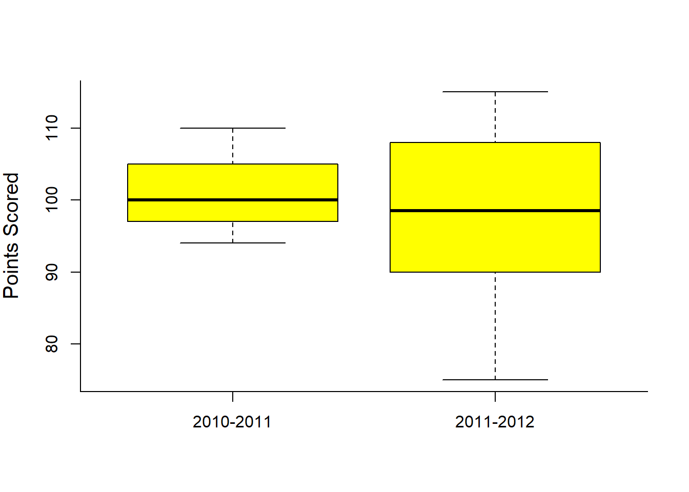

We can quickly compare the means

t.test(Year2010, Year2011)

## 
##  Welch Two Sample t-test
## 
## data:  Year2010 and Year2011
## t = 0.74832, df = 12.693, p-value = 0.4679
## alternative hypothesis: true difference in means is not equal to 0
## 95 percent confidence interval:
##  -5.871597 12.071597
## sample estimates:
## mean of x mean of y 
##     100.9      97.8

Clearly not a significant difference.
The F-statistic is jsut the ratio of the sample variances:

(S2.2010 <- var(Year2010))

## [1] 30.32222

(S2.2011 <- var(Year2011))

## [1] 141.2889

(F.obs <- S2.2010/S2.2011)

## [1] 0.2146115

It’s theoretical distribution is: F(9, 9). The vertical line represent our statistic:

curve(df(x,9,9), xlim=c(0,5))
abline(v=F.obs)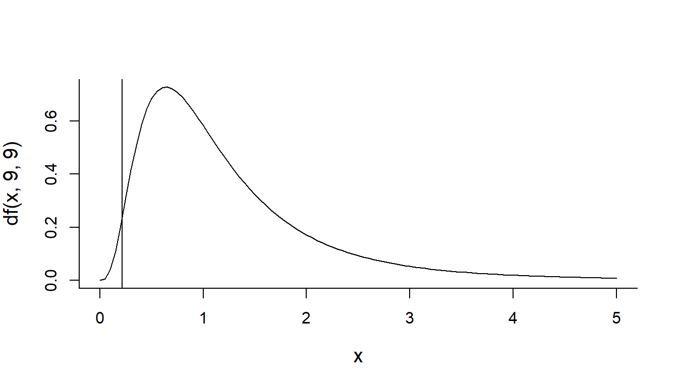

How much area is to the left of our statistic?

pf(F.obs, 9,9)

## [1] 0.0157771

I.e., a highly significant p-value, suggesting that the observed increase in variability is highly unlikely if the two sets of observations were drawn from the same process.

Exercise: Note that this test was one-sided. What if the test statistic placed 2011-2012 in the numerator, what would be the appropriate way to perform this test? How would you perform a two-sided test?

The one line way to perform this test in R is:

var.test(Year2010, Year2011)

## 
##  F test to compare two variances
## 
## data:  Year2010 and Year2011
## F = 0.21461, num df = 9, denom df = 9, p-value = 0.03155
## alternative hypothesis: true ratio of variances is not equal to 1
## 95 percent confidence interval:
##  0.05330646 0.86402470
## sample estimates:
## ratio of variances 
##          0.2146115