Lab 4: Sample spaces and counting problems
BIOL 709 / Winter 2018
Goals
The purpose of this lab is to walk through some of the basic concepts of probability theory (sample spaces, axioms of probability, counting rules) while expanding skills on manipulating and sampling vectors in R. A decent (free) text on Probability Theory and R, which might be of interest, is here: http://cran.r-project.org/web/packages/IPSUR/vignettes/IPSUR.pdf
1. Coin flipping
Flipping one coin
We can define a random variable, like our favorite simple example (the coin), by creating a vector of its sample space:
Coin <- c("H","T")Flipping a coin once is as easy as:
sample(Coin, 1)## [1] "T"Note that the sample()function rearranges any vector:
sample(1:10)## [1] 5 4 6 9 10 1 8 2 3 7And the “1” just says: take one sample.
Stealthily, sample is one of the most useful functions for a range of inference tasks - including bootstrapping and randomization tests - and for simulating various processes.
Lets say we wanted to flip 10 coins. This, doesn’t work:
sample(Coin, 10)## Error in sample.int(length(x), size, replace, prob): cannot take a sample larger than the population when 'replace = FALSE'because sample wants to rearrange Coin which only has 2 elements. So we need to “sample with replacement”:
sample(Coin, 10, replace=TRUE)## [1] "H" "T" "T" "T" "T" "H" "T" "T" "H" "H"Let’s save this object, and count the number of tails and heads:
TenCoins <- sample(Coin, 10, replace=TRUE)
table(TenCoins)
## TenCoins
## H T
## 5 5To count just the heads, for example, use the logical == (that means “is equal to”)
TenCoins == "H"## [1] FALSE FALSE TRUE TRUE FALSE FALSE TRUE TRUE TRUE FALSEsum(TenCoins == "H")## [1] 5Quick Exercise: Drawing Cards
- Create a deck with four cards: a “Club”, a “Spade”, a “Diamond” and a “Heart”.
- Sample from this deck 10 times - with replacement - and report the number of Spades in the sample.
Plot the outcome of 100 coin flips
  par(bty="l", cex.lab=1.25, las=1)
  plot(cumsum(HundredFlips == "H")/(1:length(HundredFlips)), ylim=c(0,1), type="o", ylab="Proportion heads")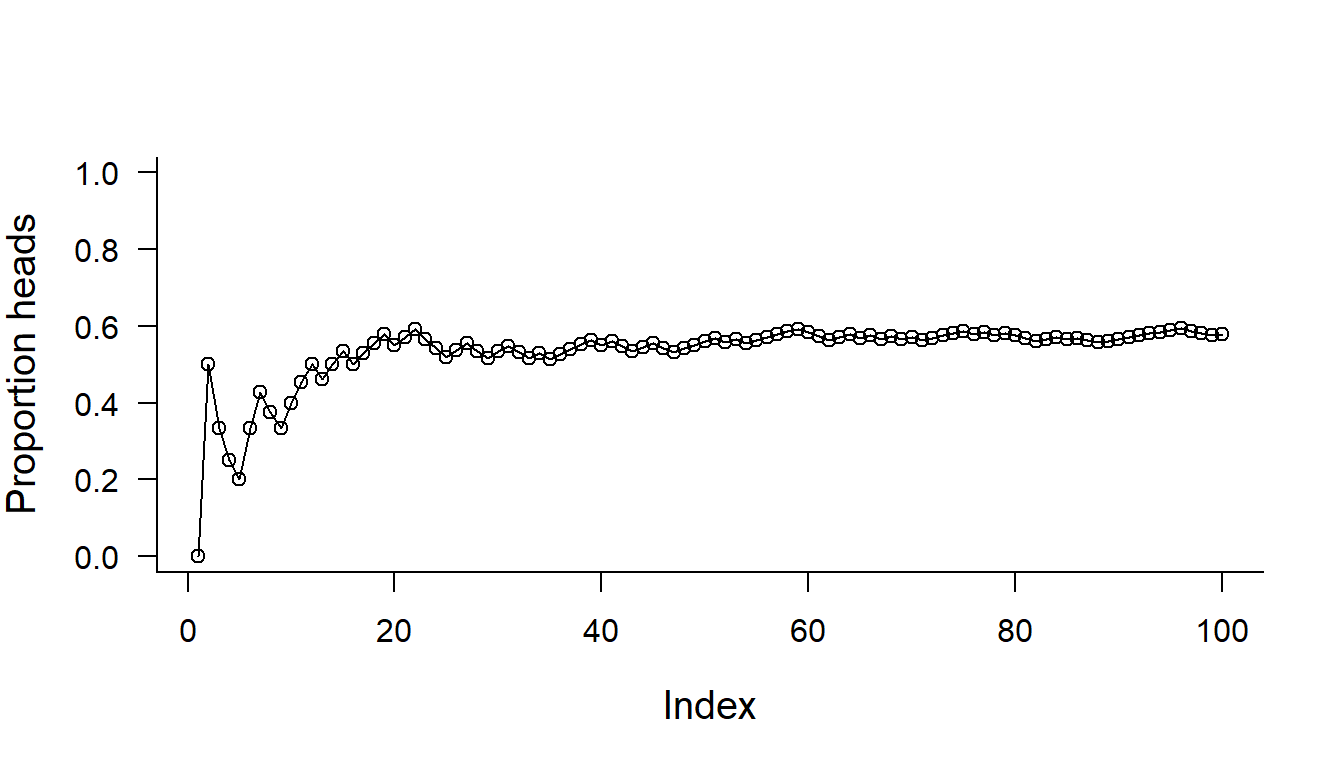
Note the use of cumsum().
Flipping 2 Coins
Let’s imagine that we flipped 2 coins, 10 times. To do that, record your first coin and second coin in two separate vectors:
CoinFlips1 <- sample(Coin, 10, replace=TRUE)
CoinFlips2 <- sample(Coin, 10, replace=TRUE)
You can see the results side by side:
data.frame(CoinFlips1, CoinFlips2)## CoinFlips1 CoinFlips2
## 1 H T
## 2 T T
## 3 H T
## 4 H H
## 5 T T
## 6 T T
## 7 H H
## 8 T H
## 9 T T
## 10 T THow many times did we flip two-of-a-kind?
CoinFlips1 == CoinFlips2## [1] FALSE TRUE FALSE TRUE TRUE TRUE TRUE FALSE TRUE TRUEgives us a vector of TRUE and FALSE. We can use sum() again:
sum(CoinFlips1 == CoinFlips2)## [1] 7How many do you EXPECT to be the same across the options?
Exercise: Coin Flips
Do this for 100 coin flips, 1000 coin flips, and 10000 coin flips. Does the proportion come closer to what you expect?
We can use paste() to combine our two coinflips to see what a double coin flip produces:
(DoubleCoinFlip <- paste(CoinFlips1, CoinFlips2, sep=""))## [1] "HT" "TT" "HT" "HH" "TT" "TT" "HH" "TH" "TT" "TT"and, of course, tabulate this result:
table(DoubleCoinFlip)## DoubleCoinFlip
## HH HT TH TT
## 2 2 1 5and also plot it:
plot(table(DoubleCoinFlip))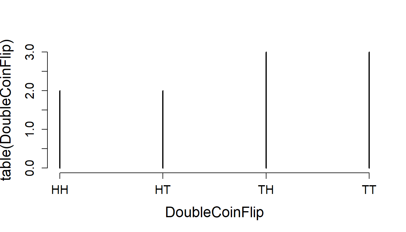
Note that the default for plotting the output of a table is a type='h' vertical bar
Question: Expectation
What do you expect the proportions to be? How would you do make this table show proportions?
Exercise: Replication
Repeat this experiment for 100 and 1000 and test your prediction.
More coin flip questions
What if we wanted to know how many of the flips had at least one head?
We use the | - which means “OR”:
CoinFlips1 == "H" | CoinFlips2 == "H"## [1] TRUE FALSE TRUE TRUE FALSE FALSE TRUE TRUE FALSE FALSEsum(CoinFlips1 == "H" | CoinFlips2 == "H")## [1] 5To count all the splits, we use the != for “Not Equal To”
CoinFlips1 != CoinFlips2## [1] TRUE FALSE TRUE FALSE FALSE FALSE FALSE TRUE FALSE FALSEsum(CoinFlips1 != CoinFlips2)## [1] 3Question: Prediction
What do you expect these proportions to be?
Exercise: Replication
Repeat this experiment for 100 and 1000 and test your prediction.
2. Simulating Dice
One die
Die <- 1:6
N <- length(Die)
Here’s a “typical” early probability problem: let “A” be the event that a roll is even, “B” that a roll is odd, and “C” that a roll is prime.
Here’s how we check for Evenness and Oddness
Die%%2 == 0## [1] FALSE TRUE FALSE TRUE FALSE TRUEA <- Die[Die%%2 == 0]
B <- Die[Die%%2 == 1]“Primeness” is trickier. I adapted some code I found online (see this post: http://www.r-bloggers.com/prime-testing-function-in-r/) and uploaded a function called isprime():
source("isprime.r")
isprime(Die)
## [1] FALSE TRUE TRUE FALSE TRUE FALSEC <- Die[isprime(Die)]The probabilites of each of these events is:
(P.even <- length(A)/N)## [1] 0.5(P.odd <- length(B)/N)## [1] 0.5(P.prime <- length(C)/N)## [1] 0.5Often it can be useful to collect these objects into a list, and apply a function across a list - using the often very handy lapply() function. See how this is done below:
lapply(list(A=A,B=B,C=C,S=Die), function(x) length(x)/length(Die))## $A
## [1] 0.5
##
## $B
## [1] 0.5
##
## $C
## [1] 0.5
##
## $S
## [1] 1Here, a list is more flexible than (e.g.) a data frame because the elements can have different lengths.
Ok, now we can ask some basic probability questions. E.g., specify the Union (OR) of each combination: (\(A \cup B, A \cup C, B \cup C\)) and the probability of each respective union (\(Pr(A \cup B), Pr(A \cup C), Pr(B \cup C)\)). This can be done by simply combining the sets and obtaining the unique elements:
(AorB <- unique(c(A,B))); length(AorB)/length(Die)## [1] 2 4 6 1 3 5## [1] 1(AorC <- unique(c(A,C))); length(AorC)/length(Die)## [1] 2 4 6 3 5## [1] 0.8333333(BorC <- unique(c(B,C))); length(BorC)/length(Die)## [1] 1 3 5 2## [1] 0.6666667Perhaps a slightly more notationally consistent way, would be to use the OR logical operator: “|”. To use that, however, we need to extract the logical vector of the original sample containing with %in%:
(AorB <-Die[(Die%in%A) | (Die%in%B)]) # even or odd## [1] 1 2 3 4 5 6(AorC <-Die[(Die%in%A) | (Die%in%C)]) # even or prime## [1] 2 3 4 5 6(BorC <-Die[(Die%in%B) | (Die%in%C)]) # odd or prime## [1] 1 2 3 5This is better in part because is easier to do the next step, which is obtain the intersections of the sets (AND): \(A \cap B, A \cap C, B \cap C\) by simply replacing the “|” with “&”:
(AandB <- Die[(Die%in%A) & (Die%in%B)]) # even and odd## integer(0)(AandC <- Die[(Die%in%A) & (Die%in%C)]) # even and prime## [1] 2(BandC <- Die[(Die%in%B) & (Die%in%C)]) # odd and prime## [1] 3 5Recall some basic probability rules: - \(P(A^c) = 1 - P(A)\) (where \(A^c\) is the complement of A) - \(P(A \cup B) = P(A) + P(B)\) if \(A\) and \(B\) are disjoint (i.e. \(A \cap B = \emptyset\)). - \(P(A \cup B) = P(A) + P(B) - P(A \cap B)\) in general - \(A\) and \(B\) are independent if \(P(A \cap B) = P(A) \times P(B)\).
We can do some quick tests of our sample spaces to see if they are disjoint or independent. First, collect all the probabilities
P.A <- length(A)/N; P.B <- length(B)/N; P.C <- length(C)/N
P.AorB <- length(AorB)/N; P.AorC <- length(AorC)/N; P.BorC <- length(BorC)/N
P.AandB <- length(AandB)/N; P.AandC <- length(AandC)/N; P.BandC <- length(BandC)/N
Test for disjiontness:
P.AorB == P.A + P.B## [1] TRUEP.AorC == P.A + P.C## [1] FALSEP.BorC == P.B + P.C## [1] FALSEOnly evens and odds are mutually exclusive.
Test for independence:
P.AandB == P.A * P.B## [1] FALSEP.AandC == P.A * P.C## [1] FALSEP.BandC == P.B * P.C## [1] FALSENone of these events are independent (not surprisingly).
3. Counting
Let’s start with a die
Die <- 1:6Make a matrix of every possible combination of two dice. This is possible with a loop, of course. But much quicker/slicker is the outer() function:
(S2Dice <- outer(Die, Die, paste))## [,1] [,2] [,3] [,4] [,5] [,6]
## [1,] "1 1" "1 2" "1 3" "1 4" "1 5" "1 6"
## [2,] "2 1" "2 2" "2 3" "2 4" "2 5" "2 6"
## [3,] "3 1" "3 2" "3 3" "3 4" "3 5" "3 6"
## [4,] "4 1" "4 2" "4 3" "4 4" "4 5" "4 6"
## [5,] "5 1" "5 2" "5 3" "5 4" "5 5" "5 6"
## [6,] "6 1" "6 2" "6 3" "6 4" "6 5" "6 6"Quick exercise: Outer
Make a similar matrix of every possible sum.
Tabulate the possible sums of a roll of two dice:
table(Sum2Dice)## Sum2Dice
## 2 3 4 5 6 7 8 9 10 11 12
## 1 2 3 4 5 6 5 4 3 2 1Make a histogram of a single die and the sum of the two dice.
plot(table(Die), col="blue", lwd=2)
plot(table(Sum2Dice), col="blue", lwd=2)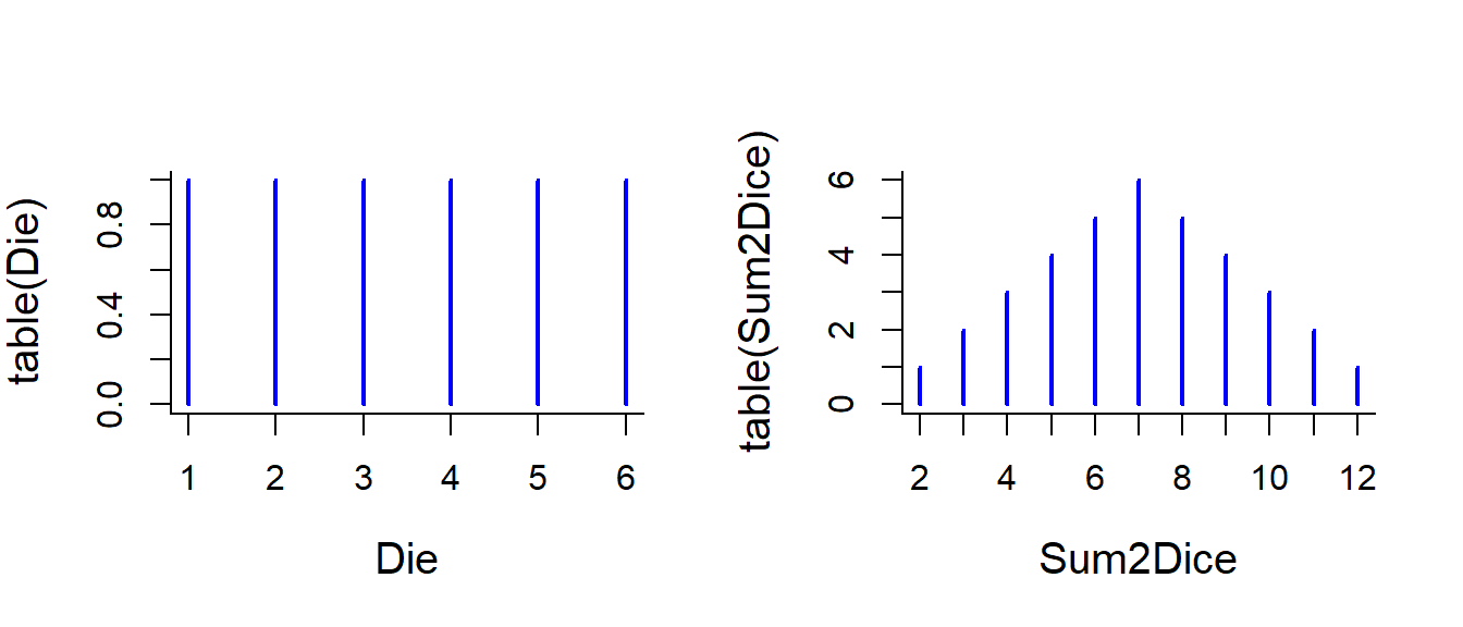
Note that - for it is not THAT straightforward to add points (pinheads) on this plot! Try: points(table(Sum2Dice)). That is because the table encodes each possible value as a discrete factor, so the 2 is a 1!
This would work:
x <- unique(as.vector(Sum2Dice))
y <- as.vector(table(Sum2Dice))
plot(x,y, type="h", lwd=2, col="blue")
points(x,y, pch=21, bg="azure", col="darkblue", cex=2, lwd=2)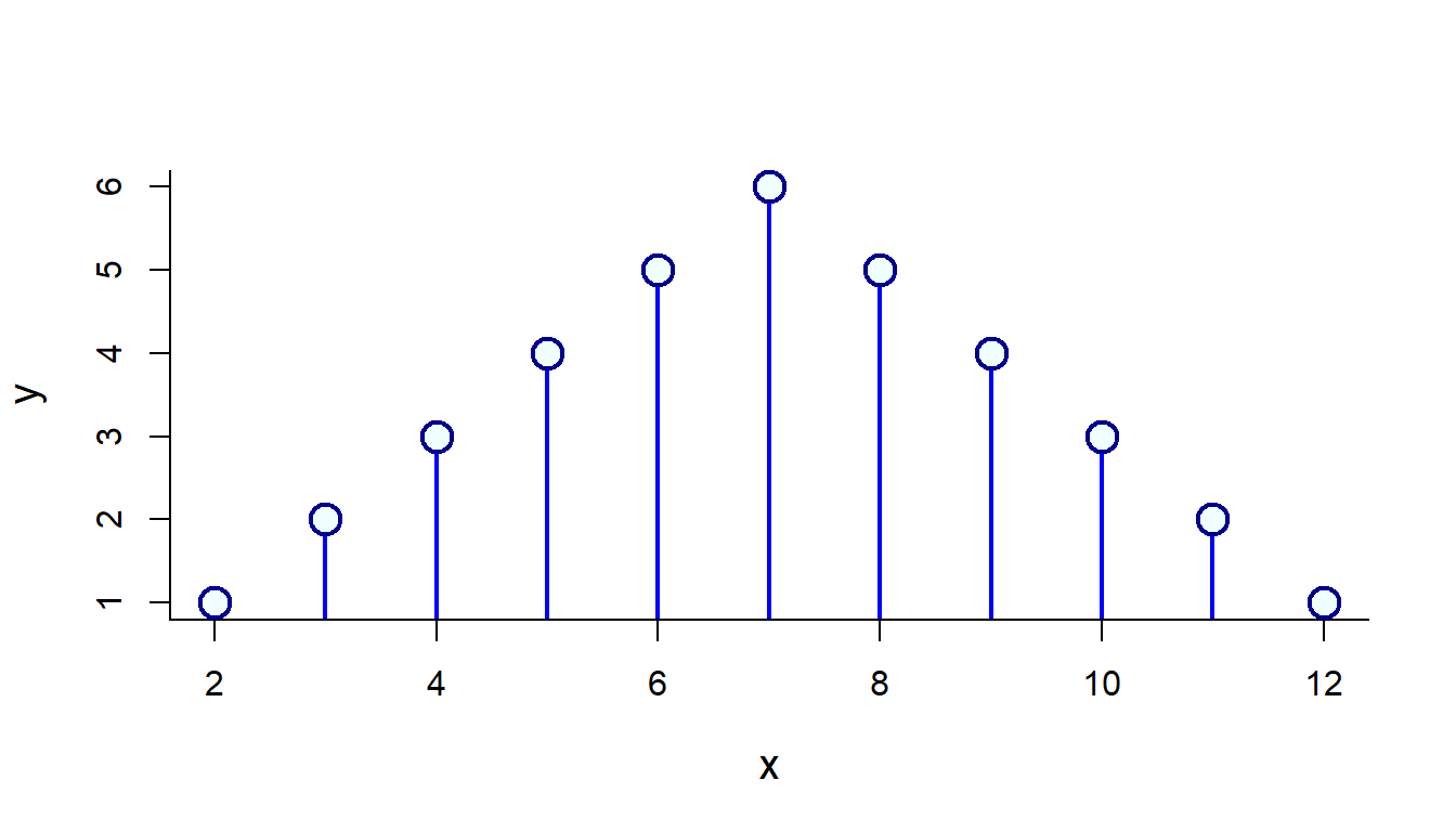
Exercise: Three Dice
Obtain the count of the sample space of the sum of three die rolls. HINT: outer() works on arrays of arbitrary dimension.
More Counting
Dinner <- c("E","F","G")
Drink <- c("B1","B2","B3")
Dessert <- c("CF","TP","SP")

DinnerCombinations <- outer(outer(Dinner, Drink, paste), Dessert, paste)
dim(DinnerCombinations)
## [1] 3 3 3length(DinnerCombinations)## [1] 27Ordering four animals
Animals <- LETTERS[1:4]There is a function in the gtools package that does combinations and permutations
require(gtools) Permute 4 animals:
permutations(4, 4, Animals)## [,1] [,2] [,3] [,4]
## [1,] "A" "B" "C" "D"
## [2,] "A" "B" "D" "C"
## [3,] "A" "C" "B" "D"
## [4,] "A" "C" "D" "B"
## [5,] "A" "D" "B" "C"
## [6,] "A" "D" "C" "B"
## [7,] "B" "A" "C" "D"
## [8,] "B" "A" "D" "C"
## [9,] "B" "C" "A" "D"
## [10,] "B" "C" "D" "A"
## [11,] "B" "D" "A" "C"
## [12,] "B" "D" "C" "A"
## [13,] "C" "A" "B" "D"
## [14,] "C" "A" "D" "B"
## [15,] "C" "B" "A" "D"
## [16,] "C" "B" "D" "A"
## [17,] "C" "D" "A" "B"
## [18,] "C" "D" "B" "A"
## [19,] "D" "A" "B" "C"
## [20,] "D" "A" "C" "B"
## [21,] "D" "B" "A" "C"
## [22,] "D" "B" "C" "A"
## [23,] "D" "C" "A" "B"
## [24,] "D" "C" "B" "A"Theoretical prediction:
factorial(4)## [1] 24- Rank (permute) 4 of 11 animals
tail(permutations(11,4,LETTERS[1:11]))## [,1] [,2] [,3] [,4]
## [7915,] "K" "J" "I" "C"
## [7916,] "K" "J" "I" "D"
## [7917,] "K" "J" "I" "E"
## [7918,] "K" "J" "I" "F"
## [7919,] "K" "J" "I" "G"
## [7920,] "K" "J" "I" "H"theoretical prediction:
factorial(11)/factorial(7)## [1] 7920Choose 4 of 11 animals:
tail(combinations(11, 4, LETTERS[1:11]))## [,1] [,2] [,3] [,4]
## [325,] "F" "I" "J" "K"
## [326,] "G" "H" "I" "J"
## [327,] "G" "H" "I" "K"
## [328,] "G" "H" "J" "K"
## [329,] "G" "I" "J" "K"
## [330,] "H" "I" "J" "K"theoretical prediction:
factorial(11)/ (factorial(7) * factorial(4))## [1] 330This is such an important quantity, it has its own “base” function
choose(11,4)## [1] 330Q1: How many unique pin-codes are possible?
Q2: How many pin codes with no repeating numbers?
4. The birthday problem
Here we will use brute simulation force to explore a probem for which (as we saw) there already is an elegant solution.
Using sample to create a class of students, assign birthdays to each one, and see if all the birthdays are unique:
ClassSize <- 30
getSharedBirthdays <- function(ClassSize)
{
  Days <- 1:365
  ClassBDays <- sample(Days, ClassSize, replace=TRUE)
  UniqueBDays <- length(unique(ClassBDays))
  ClassSize > UniqueBDays
}
getSharedBirthdays(5)
## [1] FALSEgetSharedBirthdays(30)## [1] TRUEgetSharedBirthdays(100)## [1] TRUEPerform this experiment a bunch of times
nreps <- 100
getPSharedBirthdays <- function(ClassSize, nreps)
{
  Results <- rep(NA, nreps)
  for(i in 1:nreps)
    Results[i] <- getSharedBirthdays(ClassSize)
  sum(Results)/nreps
}
getPSharedBirthdays(23, 10000)
## [1] 0.5135Perform this experiment for a range of possible class sizes:
N <- 1:70
P <- c()
for(n in N)
  P <- c(P, getPSharedBirthdays(n, 100))
plot(N,P)
abline(h=0.5) 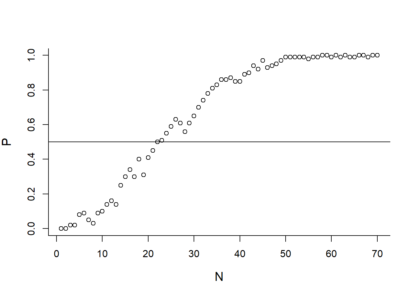
Include Theoretical prediction
Theory <- function(x)
  1 - prod(365:(365-x+1))/365^x
Theory(5)
## [1] 0.02713557Theory(23)## [1] 0.5072972Theory(100)## [1] 0.9999997But this doesn’t work:
Theory(c(5,23,100))## [1] 0.02713557 1.00000000 1.00000000What do we do? Create a loop that computes the probability for each element in a vector;
Theory2 <- function(x.vector)
{
  P <- x.vector*NA
  for(i in 1:length(x.vector))
    P[i] <- Theory(x.vector[i])
  return(P)
}
Theory2(1:50)
## [1] 0.000000000 0.002739726 0.008204166 0.016355912 0.027135574
## [6] 0.040462484 0.056235703 0.074335292 0.094623834 0.116948178
## [11] 0.141141378 0.167024789 0.194410275 0.223102512 0.252901320
## [16] 0.283604005 0.315007665 0.346911418 0.379118526 0.411438384
## [21] 0.443688335 0.475695308 0.507297234 0.538344258 0.568699704
## [26] 0.598240820 0.626859282 0.654461472 0.680968537 0.706316243
## [31] 0.730454634 0.753347528 0.774971854 0.795316865 0.814383239
## [36] 0.832182106 0.848734008 0.864067821 0.878219664 0.891231810
## [41] 0.903151611 0.914030472 0.923922856 0.932885369 0.940975899
## [46] 0.948252843 0.954774403 0.960597973 0.965779609 0.970373580OR … use the all powerful Vectorize():
Theory2 <- Vectorize(Theory)
plot(N,P)
abline(h=0.5)
lines(N, Theory2(N), lwd=2)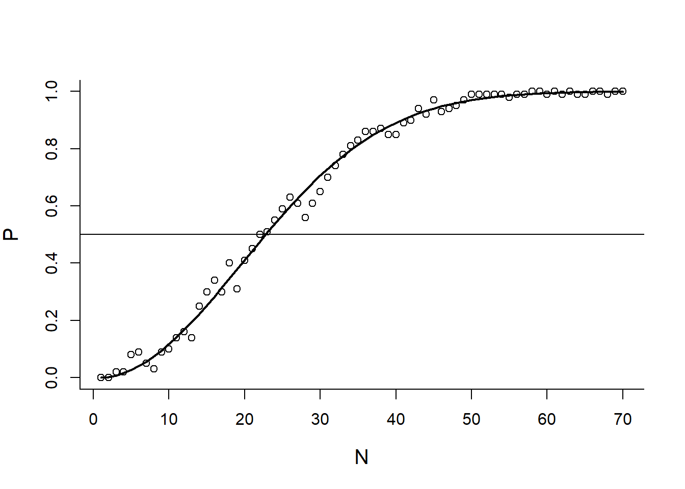
5. Distributions
Bernoulli distribution
The Bernoulli random process (\(X \sim \text{Bernoulli}(p)\)) is very similar to a coin flip, but the probability can be arbitrary (between 0 and 1), and the result is enumerated as 0 or 1. The best way to do this is using the binomial distribution, for which the Bernoulli is a special case (\(n=1\)).
rbinom(1, size=1, p=0.5)## [1] 1The r refers to “draw a random sample”, the binom refers to the distribution. This is typical for all distribution in R (we’ll talk about this more later).
We can also randomly draw a whole bunch of Bernoulli trials:
rbinom(20, size=1, p=0.3)## [1] 0 0 0 1 1 0 0 0 1 1 0 0 1 0 0 0 0 0 1 0The distribution of total number of heads after 10 coin flips
p<-0.5
x <- 0:10
choose(n, x)*p^x*(1-p)^(n-x)
## [1] 8.470329e-22 5.929231e-20 2.045585e-18 4.636658e-17 7.766403e-16
## [6] 1.025165e-14 1.110596e-13 1.015402e-12 7.996288e-12 5.508554e-11
## [11] 3.360218e-10pmf <- dbinom(x, size=10, p=0.5)
plot(x, pmf, type="h")
points(x, pmf, pch=19)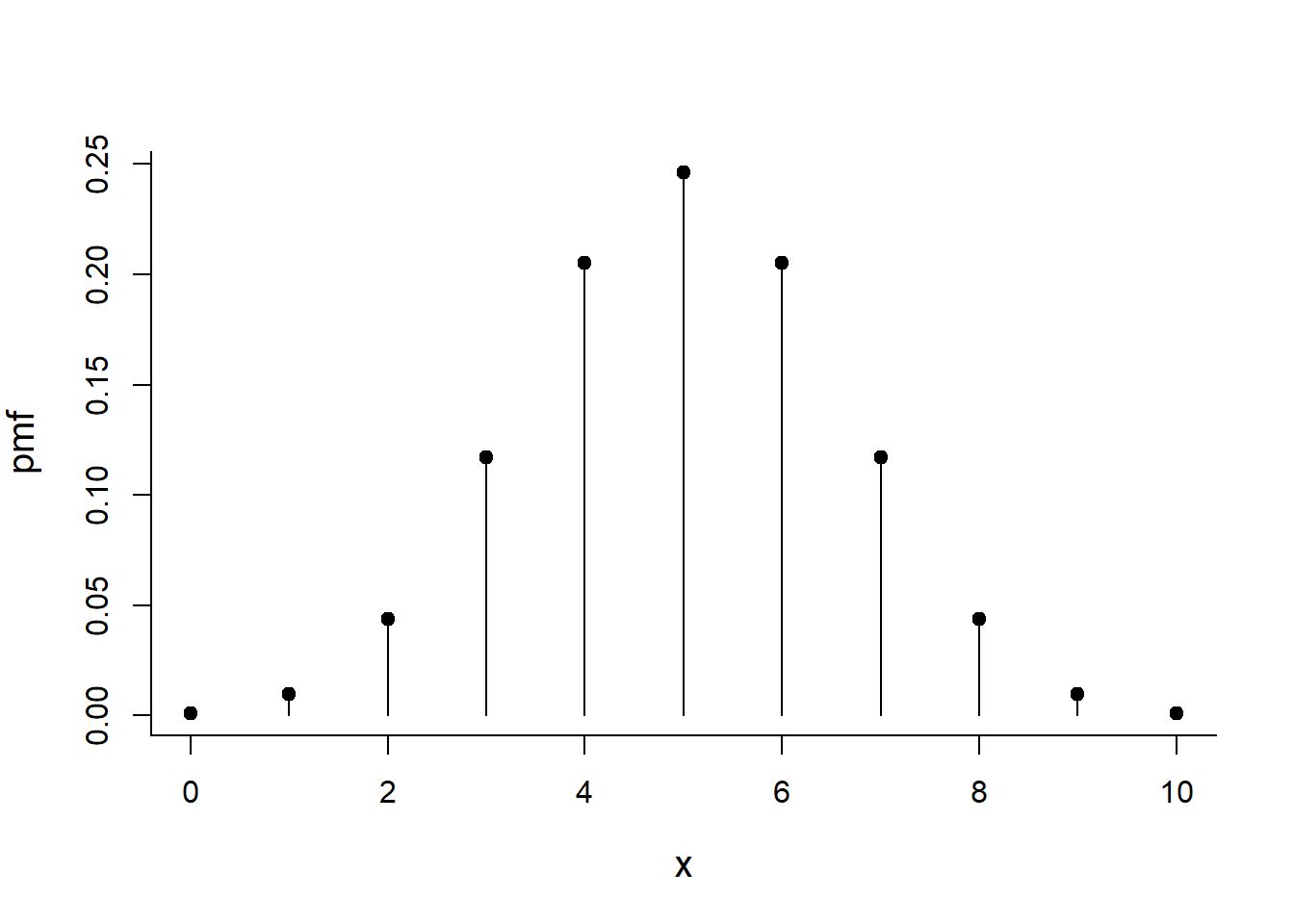
sum the pmf:
sum(pmf)## [1] 1Probability that you get exactly 5 heads
pmf[x == 5]## [1] 0.2460938Test against formula:
choose(10,5)*0.5^10## [1] 0.2460938Probability that you’ll get 6 or more heads
sum(pmf[x >= 6])## [1] 0.3769531pbinom(10,10,.5)## [1] 1Cumulative distribution
cmf <- pbinom(x, size=10, p=0.5)
plot(x, cmf, type="h")
points(x, cmf, pch=19)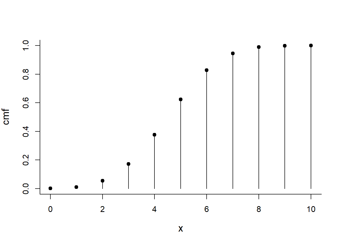
Exercise: Free throws
Given that Shaquillie O’Neal’s free throw percentage is 27%, what is the probability that he will make at least 5 of 10 critical free throws # in the last quarter of an NBA playoff game?
Random generation of binomial realizations
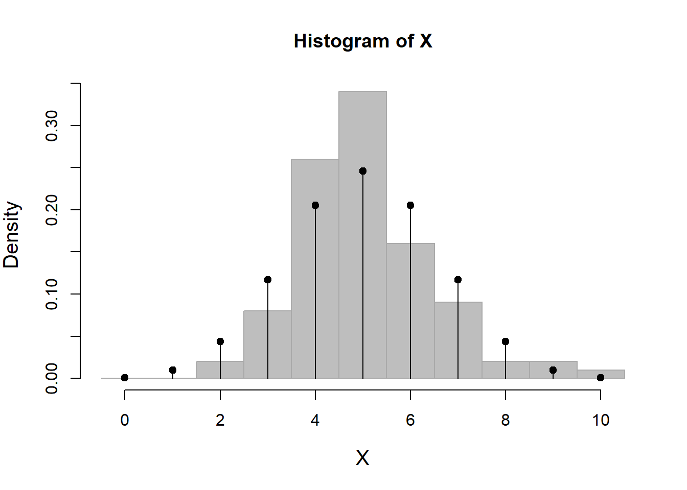
X <- rbinom(100, size=10, p=0.5)
hist(X, breaks=0:11-.5, freq=FALSE, col="grey", bor="darkgrey")
points(x, pmf, type="h")
points(x, pmf, pch=19)