Lab 3: (Quantifying) relationships between (quantitative) variables
BIOL709 / Winter 2018
Pre-loaded datasets
Iris data
There are native ways to save and access datasets within “R”. A list of “preloaded” data sets is shown with:
data()load the iris data set:
data(iris)read about it with ?iris
head(iris)## Sepal.Length Sepal.Width Petal.Length Petal.Width Species
## 1 5.1 3.5 1.4 0.2 setosa
## 2 4.9 3.0 1.4 0.2 setosa
## 3 4.7 3.2 1.3 0.2 setosa
## 4 4.6 3.1 1.5 0.2 setosa
## 5 5.0 3.6 1.4 0.2 setosa
## 6 5.4 3.9 1.7 0.4 setosasee what happens when you “plot” a data frame.
plot(iris)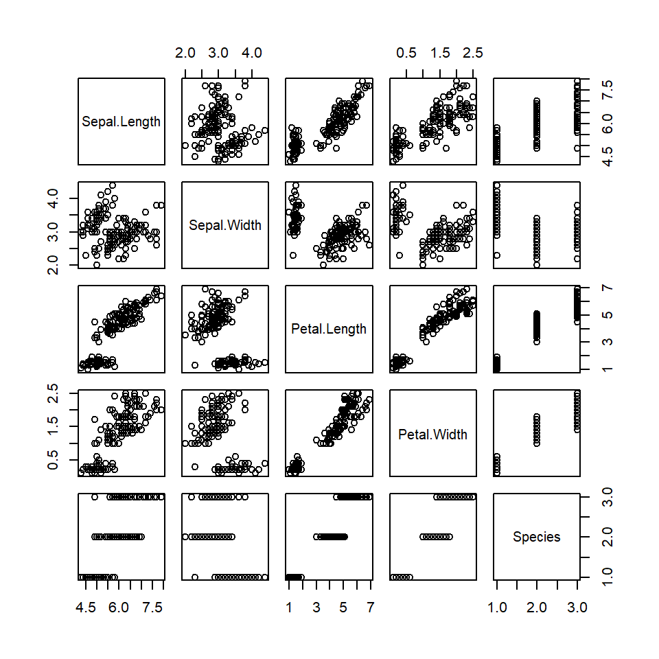
plot(iris, col=iris$Species)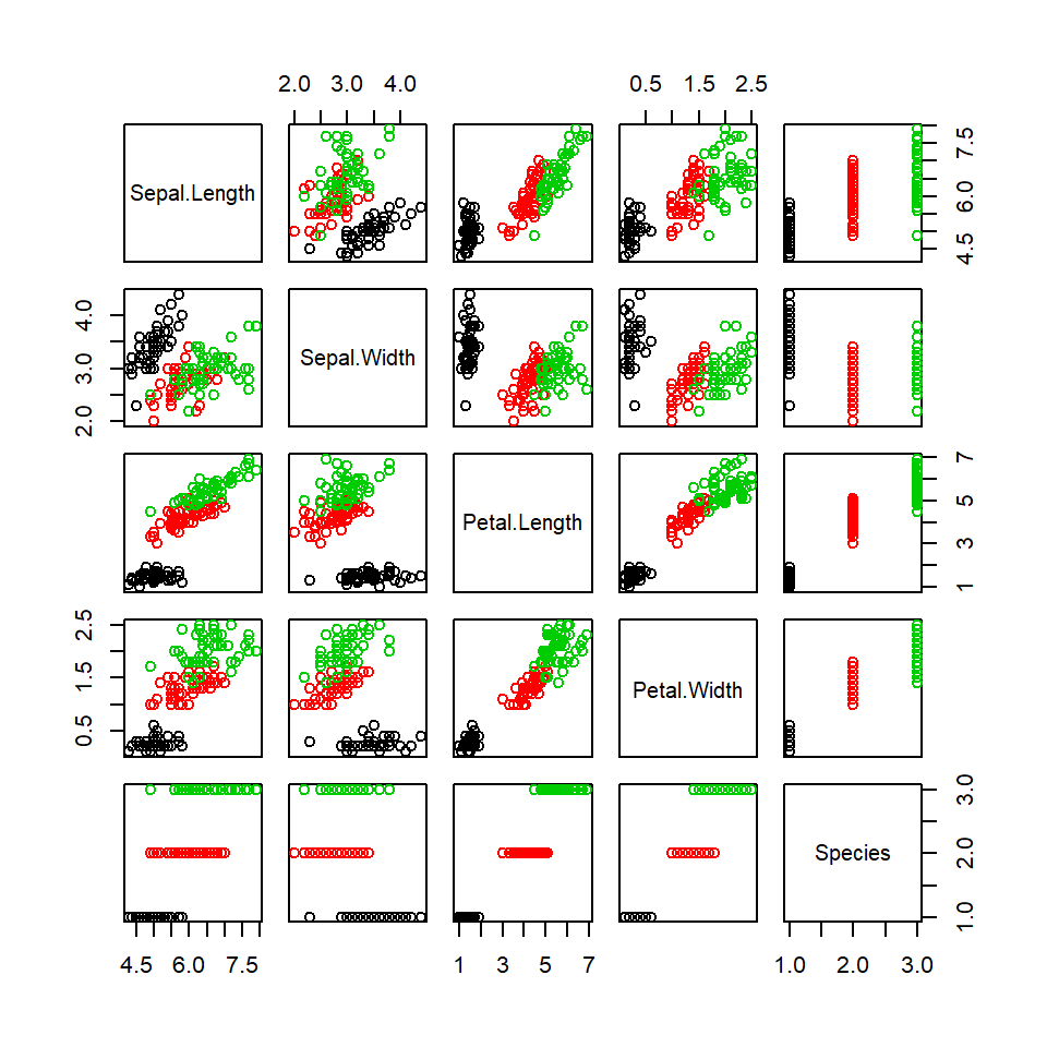
plot(iris[,1:4], col=iris$Species)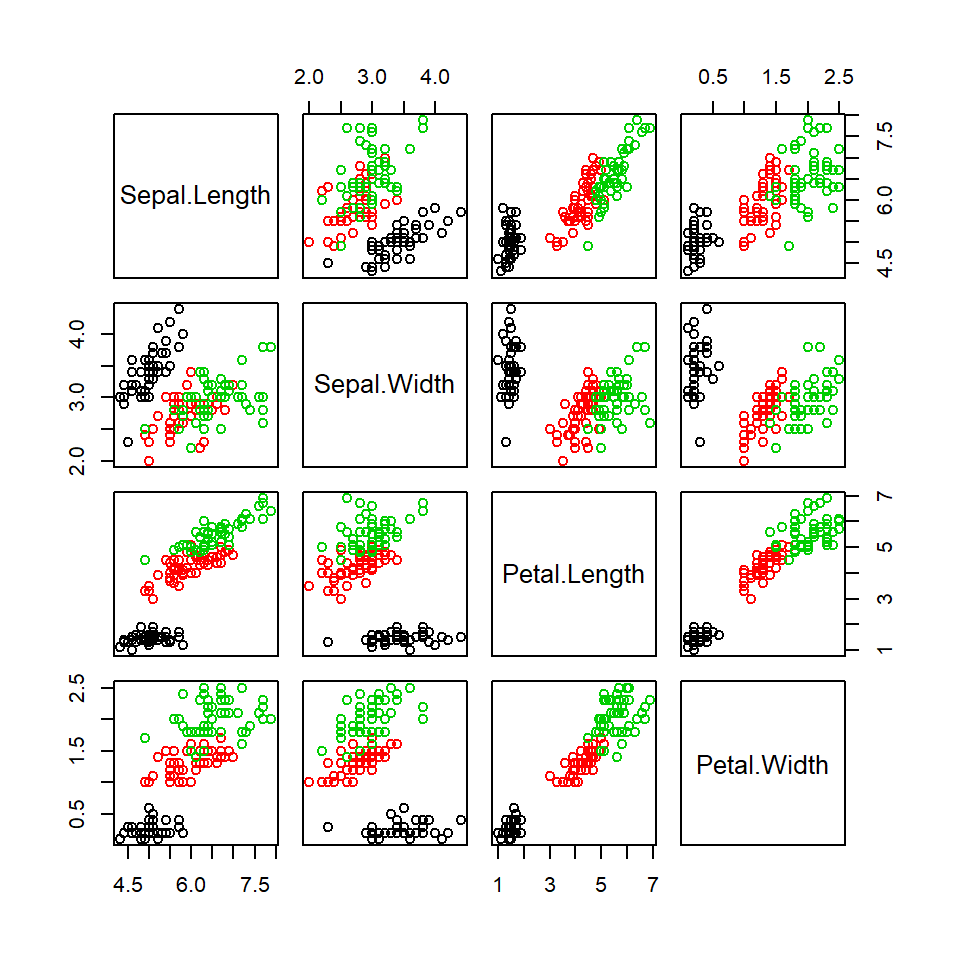
plot(iris[1:4],main="Iris Data",
    pch=21, bg=c("red","green3","blue")[iris$Species])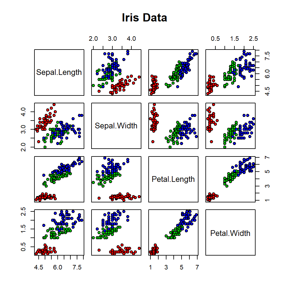
(Note the image here: http://en.wikipedia.org/wiki/Iris_flower_data_set )
Father-son data
We’d like to look at Galton’s original data. They happen to be stored in a package providing data sources for a book called UsingR. We’ll use this opportunity to install and load # a package.
Note: A “package” is a library of functions and datasets that we download / install / and use all within R. Their main repository is the CRAN website, which is mirrored around the world.
Installing a package:
install.packages("UsingR")Loading a package
library(UsingR)
require(UsingR)
Note require() simply checks if the library is already loaded, and doesn’t do anything if it is.
Loading and plotting the father.son data
data(father.son)
head(father.son)
## fheight sheight
## 1 65.04851 59.77827
## 2 63.25094 63.21404
## 3 64.95532 63.34242
## 4 65.75250 62.79238
## 5 61.13723 64.28113
## 6 63.02254 64.24221plot(father.son$fheight, father.son$sheight)
plot(father.son, pch=19, col=rgb(0,0,0,.1), asp=1)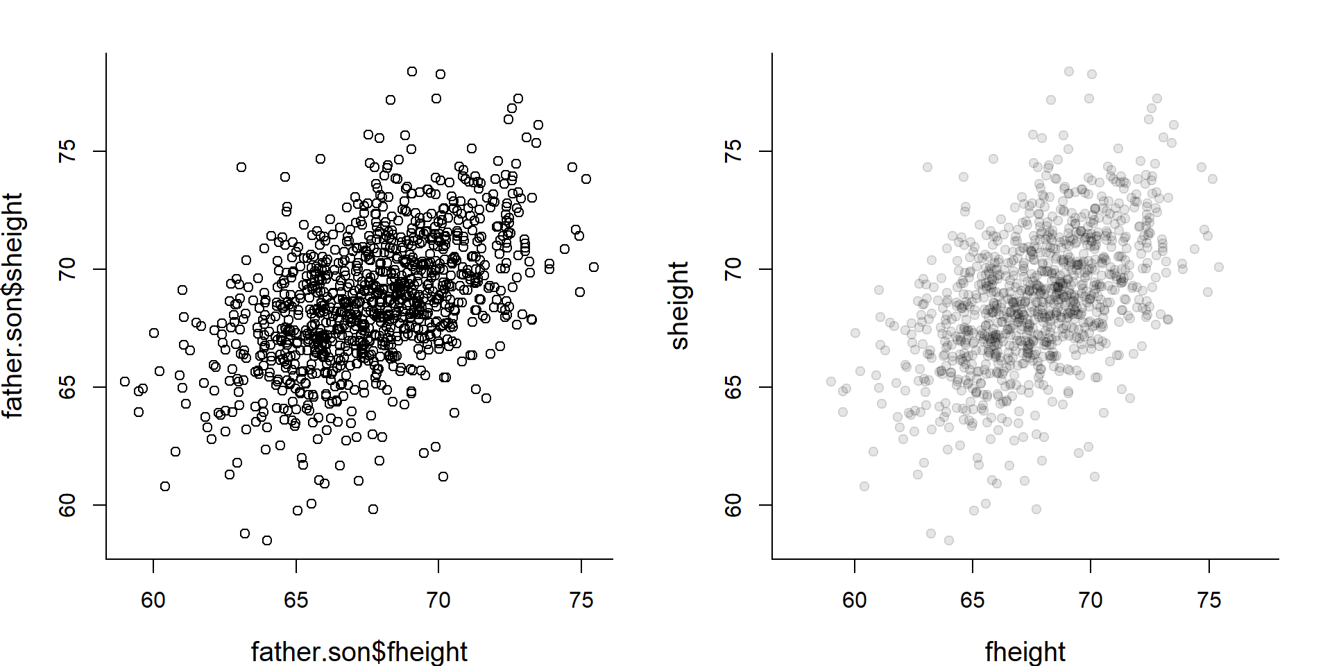
Sunflower plots
The data above are not actaully Galton’s data. Those are also present in the package, but at first glance they look less complete:
data(galton)
plot(galton)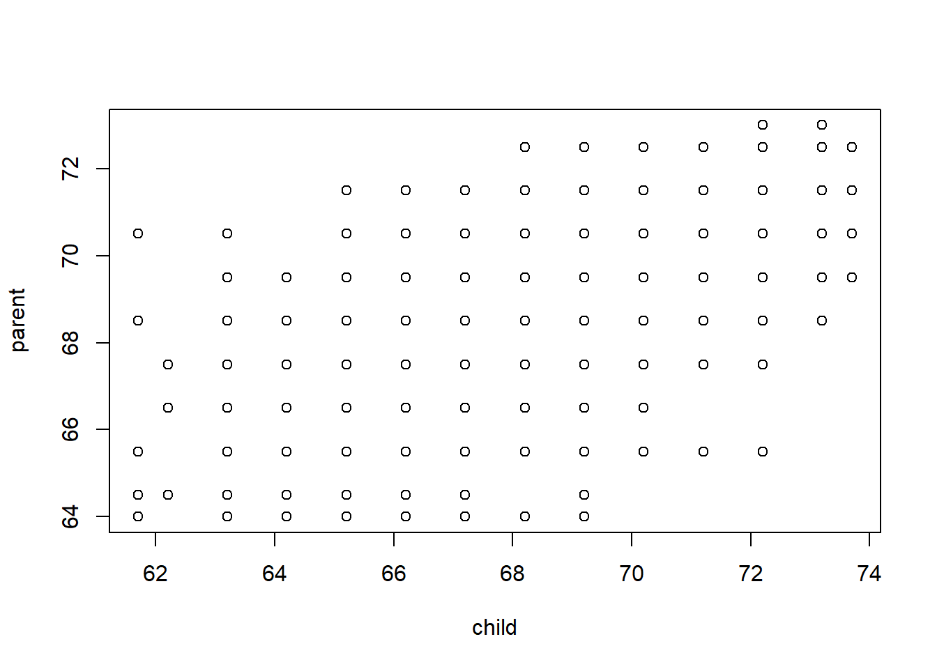
They look thin and gridded because most measurements are “discrete”, in that they were made to the centimeter or half-centimeter. We can get a better sense of the data by “jittering” and adding transparency:
data(galton)
with(galton, plot(jitter(child), jitter(parent), asp=1))
with(galton, plot(jitter(child), jitter(parent), col = rgb(0,0,0,.1), asp=1, pch = 19))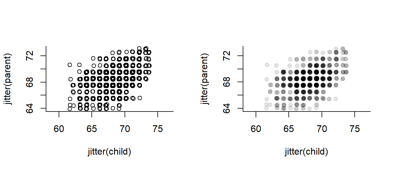 But then I discovered (just today!) an amazing thing I had never heard of before … the Sunflower Plot:
sunflowerplot(galton)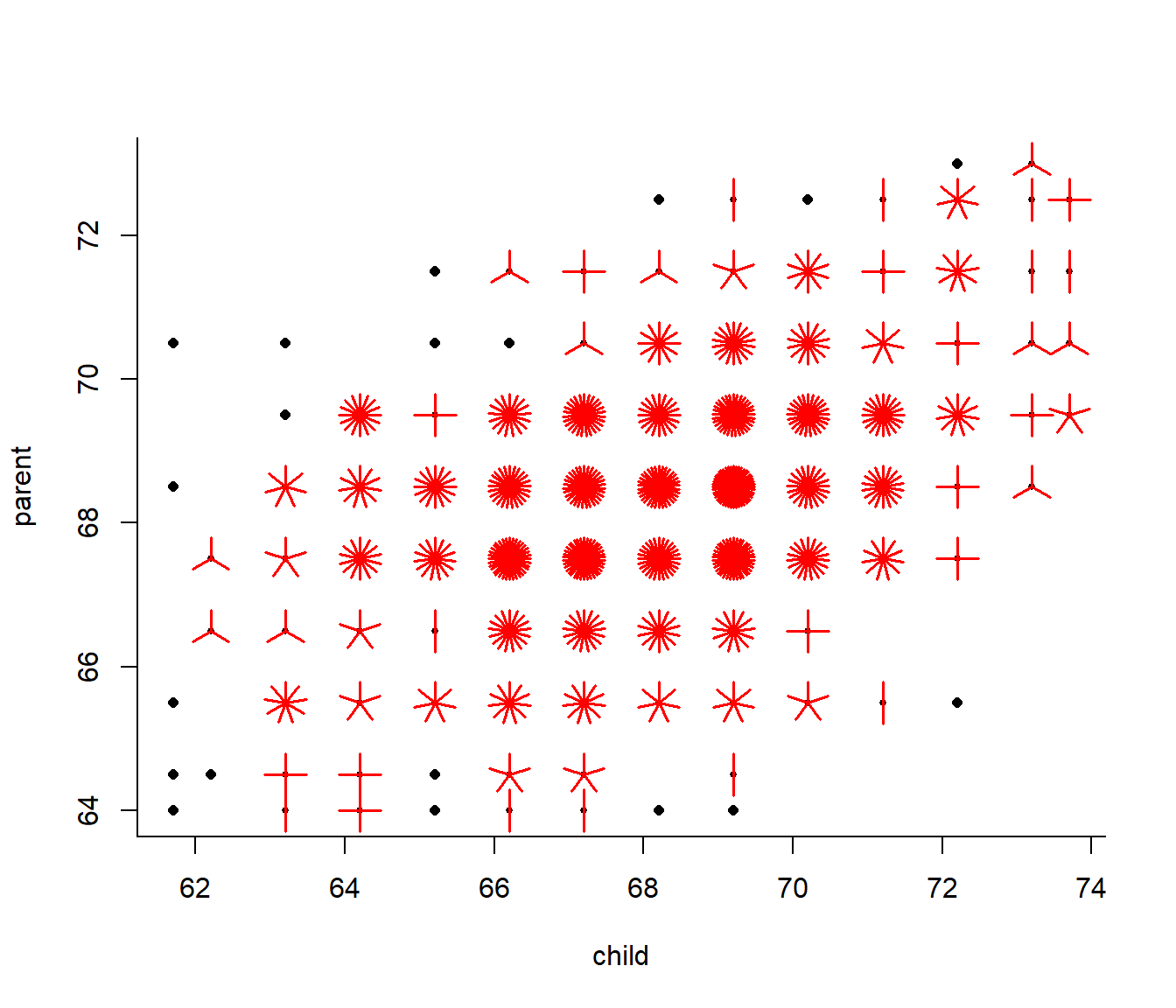
A little bit ridiculous … but why not!?
Correlations
Compute the correlation by “hand”
x <- father.son$fheight
y <- father.son$sheight
r <- sum((x-mean(x))*(y-mean(y))/(sd(x) * sd(y)))/(length(x)-1)
Compare with R’s result (predictably, the cor() function):
cor(x,y)## [1] 0.5013383cor(y,x)## [1] 0.5013383Compare with passing a matrix (or data frame) to cor
cor(father.son)## fheight sheight
## fheight 1.0000000 0.5013383
## sheight 0.5013383 1.0000000or to the covariance function:
cov(father.son)## fheight sheight
## fheight 7.534303 3.873333
## sheight 3.873333 7.922545Note that this estimates the covariance matrix \(\Sigma\) of the vector \({X_1,X_2}\), where \(i\) represents the variables, and entry \(\Sigma_{i,j} = \text{Cov}(X_i, X_i)\). A typical model for the relationship between two or more variables is the multivariate normal distribution. See the last portion of the lab for an illustration of how to visualize this distribution.
Exercise 1: Iris Correlation
Go back to the Iris data and find the correlation coefficient for all four variables. Do this for the pooled data, and then by species. Are the results consistent between species? Are there any interesting patterns between the overall correlation and the by-species correlation?
Regression coefficients
Computing the regression coefficients:
beta.hat <- sum((y-mean(y)) * (x-mean(x))) / sum((x-mean(x))^2)
alpha.hat <- mean(y) - beta.hat * mean(x)
show the relationship between \(r\), \(\widehat{\beta}\), \(s_x\) and \(s_y\).
beta.hat * (sd(x)/sd(y))## [1] 0.5013383Compute the prediction of the model, the residuals, and visualize:
y.predicted <- alpha.hat + beta.hat*x
residuals <- (y - y.predicted)
plot(y.predicted, residuals); abline(h=0, col=2)
qqnorm(residuals)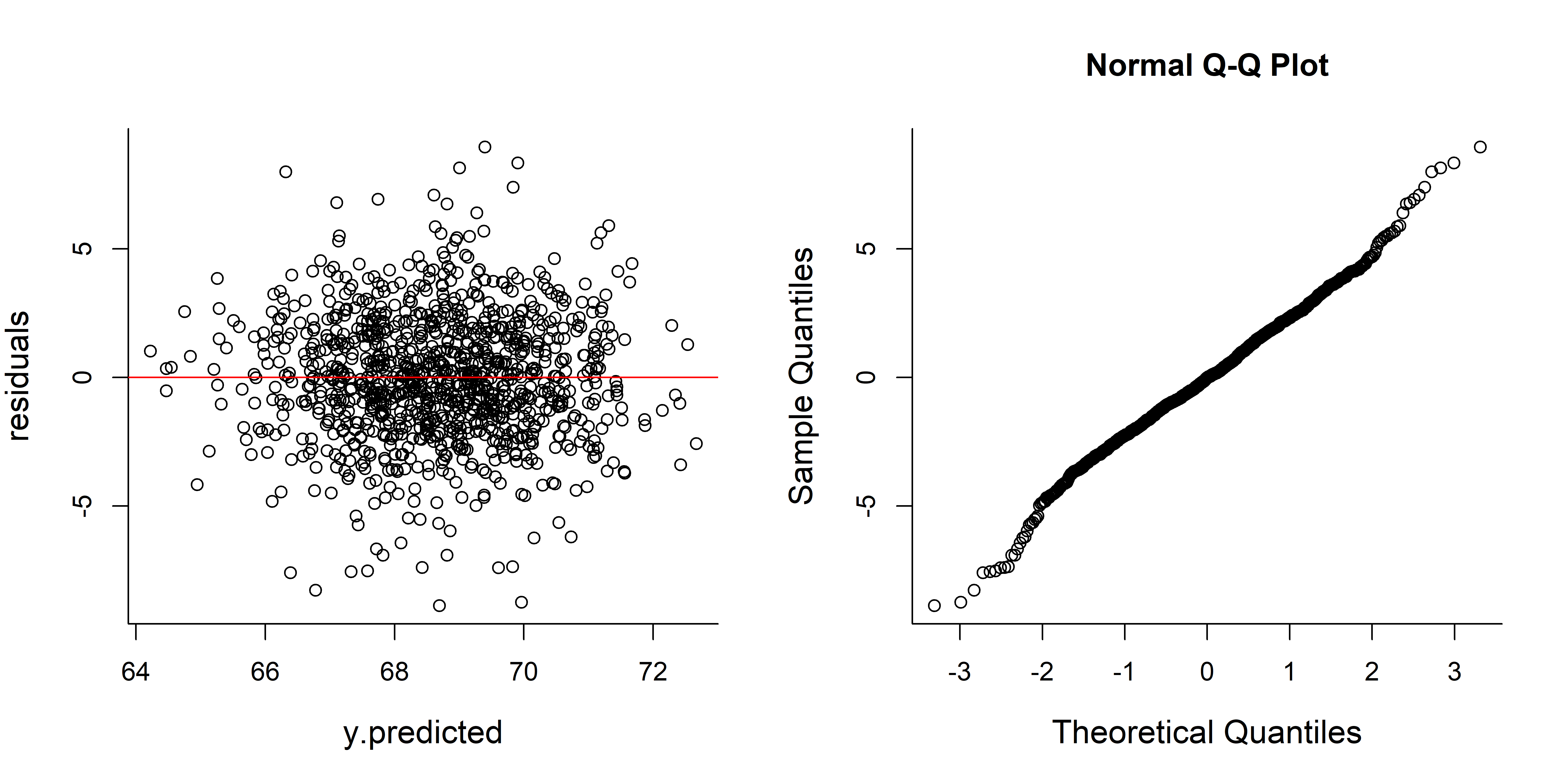
The residuals look “unstructured”, which is a good thing. And very normally distributed - also a good thing.
Compute the ancillary sums of squares:
SS.residual <- sum((y - y.predicted)^2)
SS.model <- sum( (y.predicted - mean(y))^2)
SS.total <- sum((y - mean(y))^2) # or sd(y)*(n-1)
Do they add up?
SS.residual + SS.model## [1] 8532.581SS.total ## [1] 8532.581Proportion of variation “explained” by model
SS.model/SS.total## [1] 0.2513401square root of this number:
sqrt(SS.model/SS.total)## [1] 0.5013383compare with:
r## [1] 0.5013383Linear model
And now for the (extremely important and useful) one line code for obtaining regressions: lm() - Linear Model fitting.
lm(father.son$sheight ~ father.son$fheight)##
## Call:
## lm(formula = father.son$sheight ~ father.son$fheight)
##
## Coefficients:
## (Intercept) father.son$fheight
## 33.8866 0.5141mylm <- lm(galton$child ~ galton$parent)Note, the often more compact (and recommended) way of doing this without separately “extracting” the columns:
lm(sheight ~ fheight, data=father.son)##
## Call:
## lm(formula = sheight ~ fheight, data = father.son)
##
## Coefficients:
## (Intercept) fheight
## 33.8866 0.5141The “lm” object is complex!
str(mylm)## List of 12
## $ coefficients : Named num [1:2] 23.942 0.646
## ..- attr(*, "names")= chr [1:2] "(Intercept)" "galton$parent"
## $ residuals : Named num [1:928] -7.81 -6.51 -4.57 -3.93 -3.6 ...
## ..- attr(*, "names")= chr [1:928] "1" "2" "3" "4" ...
## $ effects : Named num [1:928] -2074.19 -35.17 -4.66 -4.12 -3.86 ...
## ..- attr(*, "names")= chr [1:928] "(Intercept)" "galton$parent" "" "" ...
## $ rank : int 2
## $ fitted.values: Named num [1:928] 69.5 68.2 66.3 65.6 65.3 ...
## ..- attr(*, "names")= chr [1:928] "1" "2" "3" "4" ...
## $ assign : int [1:2] 0 1
## $ qr :List of 5
## ..$ qr : num [1:928, 1:2] -30.4631 0.0328 0.0328 0.0328 0.0328 ...
## .. ..- attr(*, "dimnames")=List of 2
## .. .. ..$ : chr [1:928] "1" "2" "3" "4" ...
## .. .. ..$ : chr [1:2] "(Intercept)" "galton$parent"
## .. ..- attr(*, "assign")= int [1:2] 0 1
## ..$ qraux: num [1:2] 1.03 1
## ..$ pivot: int [1:2] 1 2
## ..$ tol : num 1e-07
## ..$ rank : int 2
## ..- attr(*, "class")= chr "qr"
## $ df.residual : int 926
## $ xlevels : Named list()
## $ call : language lm(formula = galton$child ~ galton$parent)
## $ terms :Classes 'terms', 'formula' language galton$child ~ galton$parent
## .. ..- attr(*, "variables")= language list(galton$child, galton$parent)
## .. ..- attr(*, "factors")= int [1:2, 1] 0 1
## .. .. ..- attr(*, "dimnames")=List of 2
## .. .. .. ..$ : chr [1:2] "galton$child" "galton$parent"
## .. .. .. ..$ : chr "galton$parent"
## .. ..- attr(*, "term.labels")= chr "galton$parent"
## .. ..- attr(*, "order")= int 1
## .. ..- attr(*, "intercept")= int 1
## .. ..- attr(*, "response")= int 1
## .. ..- attr(*, ".Environment")=<environment: R_GlobalEnv>
## .. ..- attr(*, "predvars")= language list(galton$child, galton$parent)
## .. ..- attr(*, "dataClasses")= Named chr [1:2] "numeric" "numeric"
## .. .. ..- attr(*, "names")= chr [1:2] "galton$child" "galton$parent"
## $ model :'data.frame': 928 obs. of 2 variables:
## ..$ galton$child : num [1:928] 61.7 61.7 61.7 61.7 61.7 62.2 62.2 62.2 62.2 62.2 ...
## ..$ galton$parent: num [1:928] 70.5 68.5 65.5 64.5 64 67.5 67.5 67.5 66.5 66.5 ...
## ..- attr(*, "terms")=Classes 'terms', 'formula' language galton$child ~ galton$parent
## .. .. ..- attr(*, "variables")= language list(galton$child, galton$parent)
## .. .. ..- attr(*, "factors")= int [1:2, 1] 0 1
## .. .. .. ..- attr(*, "dimnames")=List of 2
## .. .. .. .. ..$ : chr [1:2] "galton$child" "galton$parent"
## .. .. .. .. ..$ : chr "galton$parent"
## .. .. ..- attr(*, "term.labels")= chr "galton$parent"
## .. .. ..- attr(*, "order")= int 1
## .. .. ..- attr(*, "intercept")= int 1
## .. .. ..- attr(*, "response")= int 1
## .. .. ..- attr(*, ".Environment")=<environment: R_GlobalEnv>
## .. .. ..- attr(*, "predvars")= language list(galton$child, galton$parent)
## .. .. ..- attr(*, "dataClasses")= Named chr [1:2] "numeric" "numeric"
## .. .. .. ..- attr(*, "names")= chr [1:2] "galton$child" "galton$parent"
## - attr(*, "class")= chr "lm"names(mylm)## [1] "coefficients" "residuals" "effects" "rank"
## [5] "fitted.values" "assign" "qr" "df.residual"
## [9] "xlevels" "call" "terms" "model"For now (while we are summarizing, not performing inference) we are mostly just interested in the coefficients
mylm$coefficients## (Intercept) galton$parent
## 23.9415302 0.6462906Note that you can access named objects with a minimally unambigious initial string of letters
mylm$coeff## (Intercept) galton$parent
## 23.9415302 0.6462906mylm$co## (Intercept) galton$parent
## 23.9415302 0.6462906# but not:
mylm$c## NULLExercise 2: Reversing the Regression
Perform the regression of children against parents. Are the coefficients the same as parents against children? How are they related?
The abline() function is useful for plotting regression lines.
par(bty="l", cex.lab=1.25)
plot(x,y, col=rgb(0,0,0,.5), pch=19)
abline(alpha.hat, beta.hat, lwd=4, col=2)
abline(mylm$coef[1], mylm$coef[2], lwd=3, col=3)
# or, most compactly,
abline(mylm, lwd=2, col=4)
#compare that to the 0,1 line
abline(0, 1, lwd=4, lty=3, col="pink")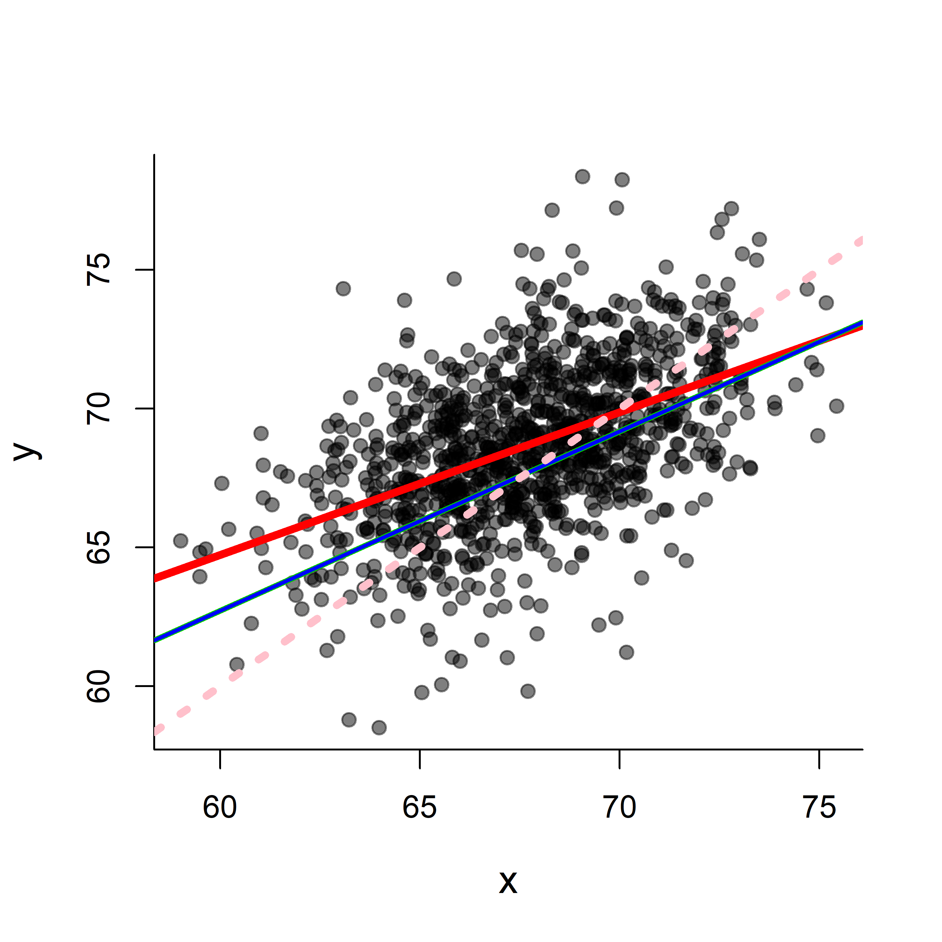
Note that a complete linear model can be fit and plotted in two very short lines of code:
plot(x,y)
abline(lm(y~x))
The summary() function is a very useful one for assessing a linear model (and, in fact, for summarizing lots of complex R objects). In particular:
summary(mylm)##
## Call:
## lm(formula = galton$child ~ galton$parent)
##
## Residuals:
## Min 1Q Median 3Q Max
## -7.8050 -1.3661 0.0487 1.6339 5.9264
##
## Coefficients:
## Estimate Std. Error t value Pr(>|t|)
## (Intercept) 23.94153 2.81088 8.517 <2e-16 ***
## galton$parent 0.64629 0.04114 15.711 <2e-16 ***
## ---
## Signif. codes: 0 '***' 0.001 '**' 0.01 '*' 0.05 '.' 0.1 ' ' 1
##
## Residual standard error: 2.239 on 926 degrees of freedom
## Multiple R-squared: 0.2105, Adjusted R-squared: 0.2096
## F-statistic: 246.8 on 1 and 926 DF, p-value: < 2.2e-16Quick Exercise: summary(lm)
Explore the “summary(lm)” object and obtain the r^2 value.
Higher order polynomial
Fitting higher order polynomials is as easy as adding that higher order as a covariate:
y <- iris$Petal.Length
x <- iris$Petal.Width
plot(x,y)
x2 <- x^2
mylm <- lm(y~x+x2)
curve(mylm$coef[1] + mylm$coef[2]*x + mylm$coef[3]*x^2, add=TRUE, col=2, lwd=2)
plot(x,mylm$residuals); abline(h=0, col=2, lwd=2)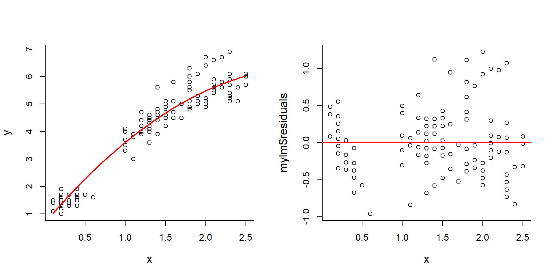
A very specific R syntax: Rather than create a new vector x2, use the I() function inside the lm function:
lm(Petal.Length ~ Petal.Width + I(Petal.Width^2), data = iris)##
## Call:
## lm(formula = Petal.Length ~ Petal.Width + I(Petal.Width^2), data = iris)
##
## Coefficients:
## (Intercept) Petal.Width I(Petal.Width^2)
## 0.6781 3.4548 -0.5277The reason you need the I is that arithmetic operators (+, -, *, ^) have a unique linear-modeling specific meaning in R’s formula definition syntax.
Exercise 3: R2 of higher order models
Obtain and compare the \(r^2\) of the simple linear model and the quadratic model. Which is likely to be higher? Does that mean that this is a “better” model? What if you added a cubic term?
Transformed data: Brain and Body Size
The animal brain and body size dataset is available in the MASS package (data sets from Modern Applied Statistics with S by Venables and Ripley - a “classic” text).
require(MASS)
data(Animals)
body <- Animals$body
brain <- Animals$brain
names <- row.names(Animals)
The following little function is handy for writing out the results of a regression:
writeRegression <- function(lm, x, y, ...)
{
  a <- lm$coef[1]
  b <- lm$coef[2]
  r2 <- summary(lm)$r.squared

  Text <- paste("Y = ", format(a, digits=3), "+", format(b, digits=3), "X \n", "R2 =", format(r2, digits=3), sep="")
  text(x, y, Text, pos = 4, ...)
}
Plotting the straightforward regression, with some text labeling of extreme animals:
plot(Animals, pch=19, col=rgb(0.8,0.2,0,.2))
text(Animals[which.max(body),], label=names[which.max(body)], cex=0.8, col="darkred", pos=2)
text(Animals[which.max(brain),], label=names[which.max(brain)], cex=0.8, col="darkred", pos=4)
text(Animals[which.min(brain),], label=names[which.min(brain)], cex=0.8, col="darkred", pos=4)
abline(lm(brain~body), lwd=3, col="darkgreen")
writeRegression(lm(brain~body), 40000, 5000, cex=1.5, col="darkred")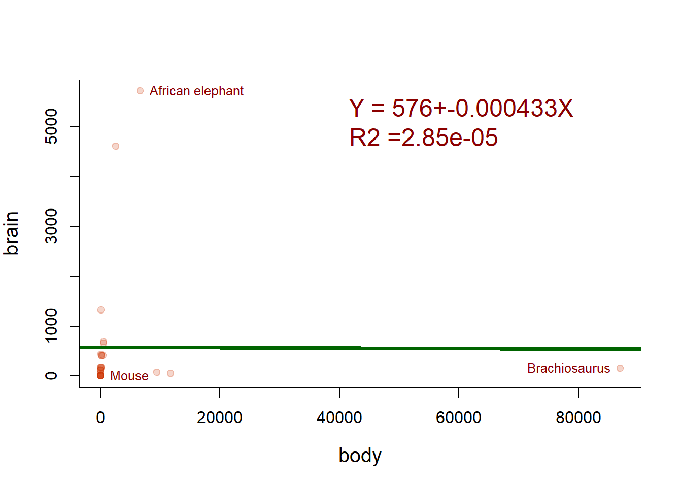
Eliminating the Brachiosaurus
plot(Animals, pch=19, col=rgb(0.8,0.2,0,.2))
text(Animals[which.max(body),], label=names[which.max(body)], cex=0.8, col="darkred", pos=2)
text(Animals[which.max(brain),], label=names[which.max(brain)], cex=0.8, col="darkred", pos=4)
text(Animals[which.min(brain),], label=names[which.min(brain)], cex=0.8, col="darkred", pos=4)
lm2 <- lm(brain~body, data=Animals[-which.max(body),])
abline(lm2, lwd=3, col="darkgreen")
writeRegression(lm2, 40000, 5000, cex=1.5, col="darkred")
Better, but not great. But how about the log-transformed data?
plot(Animals, pch=19, col=rgb(0.8,0.2,0,.2), log="xy")
text(body, brain, names, col="darkred", cex=0.8, pos=2, xpd=TRUE)
lm3 <- lm(log(brain)~log(body))
curve(exp(lm3$coef[1] + lm3$coef[2]*log(x)), add=TRUE, col="darkgreen", lwd=3, xpd=FALSE)
writeRegression(lm3, 1000, 3, cex=1.5, col="darkred")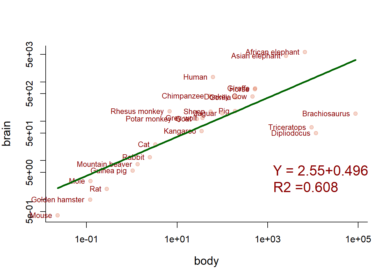
Can we clip the three dinosaur outliers?
plot(Animals, pch=19, col=rgb(0.8,0.2,0,.2), log="xy")
text(body, brain, names, col="darkred", cex=0.8, pos=2, xpd=TRUE)
lm4 <- lm(log(brain)~log(body), data=Animals, subset=body < 7500)
curve(exp(lm4$coef[1] + lm4$coef[2]*log(x)), add=TRUE, col="darkgreen", lwd=3, xpd=FALSE)
writeRegression(lm4, 1000, 3, cex=1.5, col="darkred")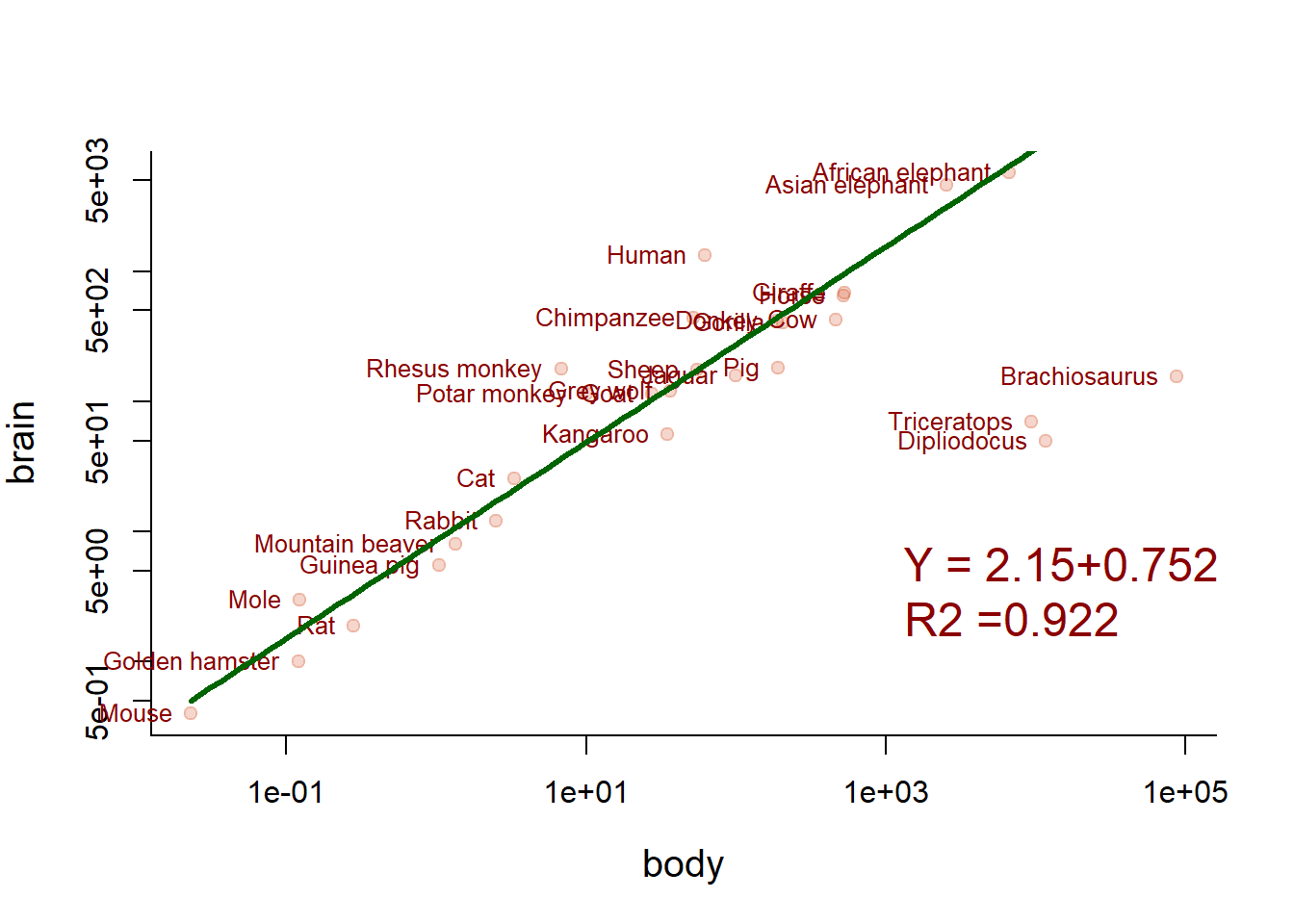
Now we’re talking! Note carefully how the fitted line is drawn.
EXTRA-TOPIC: Multivariate Normal Model
Note - This topic is totally out of place! To properly understand it you need to first properly understand what probability distribution functions are! But because I alluded to in the lecture, I go through it here.
A very widely useful model for correlated data is the multivariate normal distribution alluded to in the lecture. It can be denoted: \({\bf X} = {\cal MVN}({\bf \mu}, \Sigma)\) where \({\bf X}\) is a vector of observations, meaning that the \(i\)th observation consists of \(k\) variables: \(X_{1,i}, X_{2,i}, X_{3,i} ... X_{k,i}\), \({\bf \mu}\) is a vector of means (length \(k\)), and \(\Sigma\) is a \(k \times k\) covariance matrix. If \(k=2\), this model is known as the bivariate normal distribution and models PAIRED data (\(X,Y\)), i.e. exactly the kind of data we’ve summarized in this lab.
For the Galton data, for example, the estimates of \(\widehat{\bf \mu}\) and \(\Sigma\) are:
(mu.hat <- apply(galton, 2, mean))## child parent
## 68.08847 68.30819(Sigma.hat <- cov(galton))## child parent
## child 6.340029 2.064614
## parent 2.064614 3.194561The multivariate distribution is available in the mvtnorm package:
## install.packages("mvtnorm")
require(mvtnorm)
## Loading required package: mvtnorm##
## Attaching package: 'mvtnorm'## The following objects are masked from 'package:mixtools':
##
## dmvnorm, rmvnormTo illustrate this distribution, we need to use several moderately advanced R tricks. First, establish a range over which you’d like to visualize the distribution:
X <- seq(min(father.son$fheight), max(father.son$fheight), 0.5)
Y <- seq(min(father.son$sheight), max(father.son$sheight), 0.5)
We create a NEW function that takes “x” and “y” and returns the multivariate normal
dmvnorm2 <- Vectorize(function(x,y, ...) dmvnorm(c(x,y), ...))A few notes about this function:
- Note 1: The original “dmvnorm” needs a vector (as long as the dimensions). We’re just getting a bivariate normal, so we pass the two arguments of our functions separately, and then fill that vector
- Note 2: Very important … the “Vectorize” command that wraps around this function which works on individual values into a function that works on Vectors of values. We need this for the
outercommand to work. - Note 3: We use the “…” because it lets us pass further arguments to the function INSIDE our function without specifying all those arguments. This also works inside of functions that PASS functions (like ‘outer’).
Finally, to compute the values of the distrubution for every combination of X and Y:
MVN.matrix <- outer(X, Y, dmvnorm2, mean = mu.hat, sigma = Sigma.hat)This powerful one-liner says: Take my X values and my Y values and compute the bivariate normal distribution at each combination of those values using a mean of mu.hat and a variance-covariace of Sigma.hat
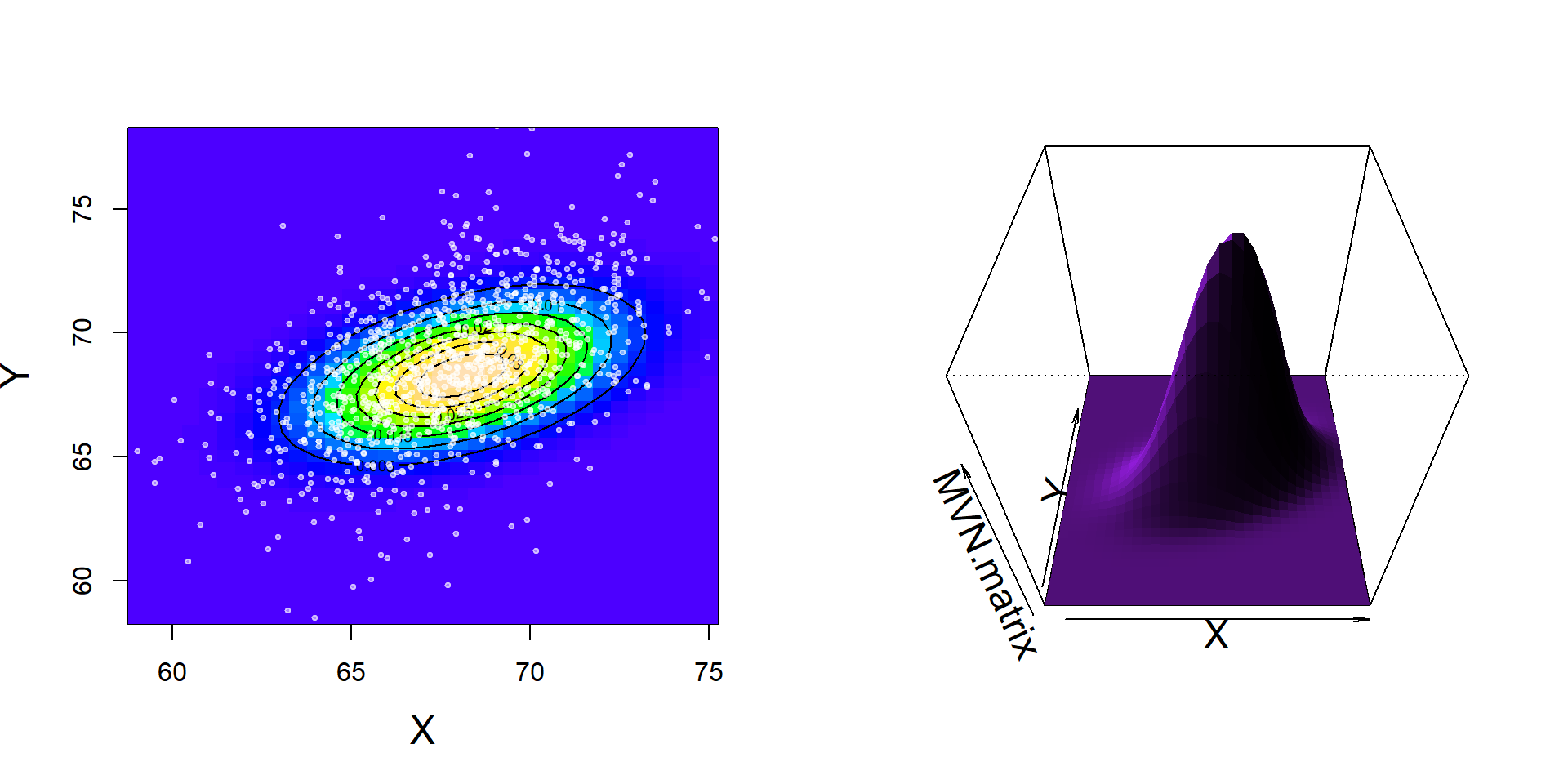
We can visualize this result as an image, contour or persp plot - all fun options:
# color coded image plot
image(X, Y, MVN.matrix, col=topo.colors(100))
contour(X, Y, MVN.matrix, add=TRUE)
points(father.son, pch=19, cex=0.5, col=rgb(1,1,1,0.5))
#3D surface plot
persp(X,Y,MVN.matrix, shade=TRUE, theta = 0, phi = 45, border=NA, col="purple")