Lab 2: Summary Statistics (and more visualizations)
BIOL709 / Winter 2018
Summarizing Quantitative data
Load the sealion data, whether locally or from the web:
## Sealion <- read.csv("../_data/PupTaggingData.csv")
Sealion <- read.csv("https://terpconnect.umd.edu/~egurarie/teaching/Biol709/data/PupTaggingData.csv")
“Extract” the colums into separate vectors.
Length <- Sealion$Length
Girth <-Sealion$Girth
Weight <-Sealion$Weight
Island <- Sealion$Island
Sex <- Sealion$Sex
Some of the quantitative summary statistics we learned are:
mean(Length)## [1] 109.8434var(Length)## [1] 34.82854sd(Length)## [1] 5.901571These are straightforward arithmetic statistics, that we could recreate ourselves if we wanted to. Thus:
Length.mean <- sum(Length)/length(Length)
Length.var <- sum((Length-Length.mean)^2)/(length(Length) - 1)
Length.sd <- sqrt(Length.var)
Other statistics are extracted from an ordering of the data, like:
range(Length)## [1] 93 126median(Length)## [1] 110quantile(Length)## 0% 25% 50% 75% 100%
## 93.00 106.00 110.00 114.75 126.00The quantile function, by default, gives the 0, 25, 50, 75 and 100th percentiles. The most practically useful uses for quantile are to get the interquantile range (IQR), and - later, when we talk about confidence intervals - the 2.5% and 97.5% percentiles.
quantile(Length, prob = c(.25,.75))## 25% 75%
## 106.00 114.75quantile(Length, prob = c(.025,.975))## 2.5% 97.5%
## 98 121Note that:
min(Length) == sort(Length)[1]## [1] TRUEmax(Length) == sort(Length)[length(Length)]## [1] TRUErange(Length) == quantile(Length, c(0,1))## 0% 100%
## TRUE TRUEA Summary function
Lets make a specialized function that returns all of these statistics. Before we start, lets introduce the “list”. A “list” is a type of object that collects in it any number of distinct objects. For example:
MyPet <- list(name = "Bartholemew",
species = factor("Guinea Pig", levels=c("Dog", "Cat", "Parakeet", "Guinea Pig")),
age=4,
whiskers = TRUE,
colors = c("Tan", "White", "Black"))we access any of these elements with the “$” operator
MyPet$whiskers## [1] TRUENow, we create a function.
Every function is assigned, like any other object, with a name and some optional arguments
MySummary <- function(X){
X.mean <- sum(X)/length(X)
X.var <- sum((X-X.mean)^2)/(length(X) - 1)
X.sd <- sqrt(X.var)
list(N = length(X), range = range(X), mean = X.mean,
median = median(X), quantile = quantile(X))
}
MySummary(Length)## $N
## [1] 498
##
## $range
## [1] 93 126
##
## $mean
## [1] 109.8434
##
## $median
## [1] 110
##
## $quantile
##     0%    25%    50%    75%   100%
## 93.00 106.00 110.00 114.75 126.00MySummary(Length[Island == "Chirpoev"])## $N
## [1] 99
##
## $range
## [1] 93 121
##
## $mean
## [1] 109.9798
##
## $median
## [1] 110
##
## $quantile
## 0% 25% 50% 75% 100%
## 93.0 105.5 110.0 115.0 121.0Summarizing things by hand
Often, we want to summarize these statistics for separate subgroups. We can do that by hand, like this:
Length.Chirpoev <- mean(Length[Island == "Chirpoev"])
Length.Antsiferov <- mean(Length[Island == "Antsiferov"])
Length.Lovushki <- mean(Length[Island == "Lovushki"])

mean(Length[Island == "Chirpoev"])
## [1] 109.9798mean(Length[Island == "Antsiferov"])## [1] 110.57mean(Length[Island == "Lovushki"])## [1] 109.38mean(Length[Island == "Lovushki" & Sex == "M"])## [1] 112.3etc … but that can get quite tedious.
The tapply function
A very useful solution is to use the “tapply” function.
 tapply(Y, X, FUN):
#    1) Y is the thing you want to summarzie
#    2) X is the factor you want to organize by
#    3) FUN is the function you want to apply
tapply(Length, Island, mean)## Antsiferov Chirpoev Lovushki Raykoke Srednova
## 110.5700 109.9798 109.3800 110.7600 108.5152Note that you can specify your own function
sd.pop <- function(x)
  1/length(x) * sum((x-mean(x))^2)
tapply(Length, Island, sd.pop)
## Antsiferov Chirpoev Lovushki Raykoke Srednova
## 35.42510 37.02989 34.61560 28.28240 35.11846Or define it within the function
tapply(Length, Island, function(x) 1/length(x) * sum((x-mean(x))^2))## Antsiferov Chirpoev Lovushki Raykoke Srednova
## 35.42510 37.02989 34.61560 28.28240 35.11846Combining outputs of tapply is extremely useful for making summary tables
  SummaryTable <- data.frame(
      n = tapply(Length, Island, length),
      mean = tapply(Length, Island, mean),
      sd = tapply(Length, Island, sd))
What if we were curious about differences between sexes as well?
Here, we can combine the two factors (Island and Sex) using the very useful paste() function.
See:
  gift <- "Partridge in a Pear Tree"
  n <- 1
  paste(n, gift)
## [1] "1 Partridge in a Pear Tree" gifts <- c("French Hens", "Turtle Doves", gift)
ns <- 3:1
paste(ns, gifts)## [1] "3 French Hens" "2 Turtle Doves"
## [3] "1 Partridge in a Pear Tree" tapply(Length, paste(Island, Sex), length)## Antsiferov F Antsiferov M Chirpoev F Chirpoev M Lovushki F
## 38 62 43 56 50
## Lovushki M Raykoke F Raykoke M Srednova F Srednova M
## 50 49 51 46 53A summary table using paste
  SummaryTable <- data.frame(
    n = tapply(Length, paste(Island, Sex), length),
    mean = tapply(Length, paste(Island, Sex), mean),
    sd = tapply(Length, paste(Island, Sex), sd))
  SummaryTable
## n mean sd
## Antsiferov F 38 107.0526 4.837619
## Antsiferov M 62 112.7258 5.607867
## Chirpoev F 43 106.8605 5.383314
## Chirpoev M 56 112.3750 5.574495
## Lovushki F 50 106.4600 4.046717
## Lovushki M 50 112.3000 6.071849
## Raykoke F 49 108.1429 4.734624
## Raykoke M 51 113.2745 4.677942
## Srednova F 46 104.9348 4.454222
## Srednova M 53 111.6226 5.339355Note: this summary table doesn’t have a separate column for “Island” and “Sex” … how might you make one?
The “tapply” is part of a family of “apply” functions, which can be a bit confusing, but are often quite useful.
We will use “tapply” and “apply” to make a summary table that combines both
  M <- matrix(tapply(Length, paste(Sex, Island), mean), nrow=length(levels(Island)))
  rownames(M) <- levels(Island)
  colnames(M) <- levels(Sex)
apply(Y, MAR, FUN) applies function FUN to variable Y across a “margin” (1 = by rows, 2 = by columnd)
  MeansByIsland <- apply(M, 1, mean)
  MeansBySex <- apply(M, 2, mean)

  SummaryTable <- data.frame(M, Total = MeansByIsland)
  SummaryTable <- rbind(SummaryTable, Total = apply(SummaryTable, 2, mean))
  SummaryTable
## F M Total
## Antsiferov 107.0526 112.7258 109.8892
## Chirpoev 106.8605 112.3750 109.6177
## Lovushki 106.4600 112.3000 109.3800
## Raykoke 108.1429 113.2745 110.7087
## Srednova 104.9348 111.6226 108.2787
## Total 106.6901 112.4596 109.5749According to this table - the mean of the means is 109.57, whereas:
mean(Length) # gives 109.84. ## [1] 109.8434Why the difference?
Note that if the function returns a vector, the output of tapply becomes a “list”
tapply(Length, paste(Island,Sex), quantile)## $`Antsiferov F`
## 0% 25% 50% 75% 100%
## 96.00 104.25 106.50 109.75 117.00
##
## $`Antsiferov M`
## 0% 25% 50% 75% 100%
## 95.00 109.25 114.00 117.00 125.00
##
## $`Chirpoev F`
## 0% 25% 50% 75% 100%
## 97.0 103.5 106.0 110.0 121.0
##
## $`Chirpoev M`
## 0% 25% 50% 75% 100%
## 93.00 108.75 114.00 116.00 121.00
##
## $`Lovushki F`
## 0% 25% 50% 75% 100%
## 96.00 105.00 107.00 109.75 114.00
##
## $`Lovushki M`
## 0% 25% 50% 75% 100%
## 97.00 109.00 111.50 115.75 126.00
##
## $`Raykoke F`
## 0% 25% 50% 75% 100%
## 99 105 108 111 119
##
## $`Raykoke M`
## 0% 25% 50% 75% 100%
## 105 110 113 117 122
##
## $`Srednova F`
## 0% 25% 50% 75% 100%
## 94.00 102.00 105.00 107.75 116.00
##
## $`Srednova M`
## 0% 25% 50% 75% 100%
## 100 108 112 115 121there is another, related, function called “aggregate” which provides more usable output.
aggregate(Length, list(Island, Sex), quantile)## Group.1 Group.2 x.0% x.25% x.50% x.75% x.100%
## 1 Antsiferov F 96.00 104.25 106.50 109.75 117.00
## 2 Chirpoev F 97.00 103.50 106.00 110.00 121.00
## 3 Lovushki F 96.00 105.00 107.00 109.75 114.00
## 4 Raykoke F 99.00 105.00 108.00 111.00 119.00
## 5 Srednova F 94.00 102.00 105.00 107.75 116.00
## 6 Antsiferov M 95.00 109.25 114.00 117.00 125.00
## 7 Chirpoev M 93.00 108.75 114.00 116.00 121.00
## 8 Lovushki M 97.00 109.00 111.50 115.75 126.00
## 9 Raykoke M 105.00 110.00 113.00 117.00 122.00
## 10 Srednova M 100.00 108.00 112.00 115.00 121.00EXERCISE 1: A Summary Function
Write a function that returns a vector with “n”, “mean”, and “sd”, and. Use “aggregate” to create the same table as in the last exercise (basically in one line.
##       Group.1 Group.2        x.n     x.mean       x.sd
## 1  Antsiferov       F  38.000000 107.052632   4.837619
## 2    Chirpoev       F  43.000000 106.860465   5.383314
## 3    Lovushki       F  50.000000 106.460000   4.046717
## 4     Raykoke       F  49.000000 108.142857   4.734624
## 5    Srednova       F  46.000000 104.934783   4.454222
## 6  Antsiferov       M  62.000000 112.725806   5.607867
## 7    Chirpoev       M  56.000000 112.375000   5.574495
## 8    Lovushki       M  50.000000 112.300000   6.071849
## 9     Raykoke       M  51.000000 113.274510   4.677942
## 10   Srednova       M  53.000000 111.622642   5.339355
Note that this data.frame is a bit strange:
  dim(SummaryTable.Final)
  is(SummaryTable.Final[,3])
  data.frame(SummaryTable.Final[,3])
The ply functions
The tapply function, these days, is considered somewhat “old school”. Following the philosophy that we don’t actually want to break up our data frame ever, we can use the xxply family of functions in the plyr packages.
These functions (like almost all functions that emerge from Hadley Wickham’s savant R brain trust) takes a complete data set as the main parameter and modifies it as needed. The ddply function takes a data frame and returns a data frame, dlply takes a data frame and returns a list, ldply takes a list and returns a list, etc. A complete schematized is below:

The mean of length by islands:
require(plyr)
ddply(Sealion, 'Island', function(df) mean(df$Length))
## Island V1
## 1 Antsiferov 110.5700
## 2 Chirpoev 109.9798
## 3 Lovushki 109.3800
## 4 Raykoke 110.7600
## 5 Srednova 108.5152The mean of length by islands and sex:
ddply(Sealion, c('Island', 'Sex'), function(df) mean(df$Length))## Island Sex V1
## 1 Antsiferov F 107.0526
## 2 Antsiferov M 112.7258
## 3 Chirpoev F 106.8605
## 4 Chirpoev M 112.3750
## 5 Lovushki F 106.4600
## 6 Lovushki M 112.3000
## 7 Raykoke F 108.1429
## 8 Raykoke M 113.2745
## 9 Srednova F 104.9348
## 10 Srednova M 111.6226The mean and s.d. of length by islands and sex:
ddply(Sealion, c('Island', 'Sex'),
    function(df) data.frame(mean = mean(df$Length),
                                                    sd = sd(df$Length)))
## Island Sex mean sd
## 1 Antsiferov F 107.0526 4.837619
## 2 Antsiferov M 112.7258 5.607867
## 3 Chirpoev F 106.8605 5.383314
## 4 Chirpoev M 112.3750 5.574495
## 5 Lovushki F 106.4600 4.046717
## 6 Lovushki M 112.3000 6.071849
## 7 Raykoke F 108.1429 4.734624
## 8 Raykoke M 113.2745 4.677942
## 9 Srednova F 104.9348 4.454222
## 10 Srednova M 111.6226 5.339355If you have a complicated function that requires combining multiple columns of data, it is useful to write a separate function that does this. But the syntax for the simple functions is bit awkward. To the rescue comes summarize:
ddply(Sealion, c("Island", "Sex"), summarize,
            L.mean = mean(Length), L.sd = sd(Length),
            W.mean = mean(Weight), W.sd = sd(Weight))
## Island Sex L.mean L.sd W.mean W.sd
## 1 Antsiferov F 107.0526 4.837619 30.76316 4.202214
## 2 Antsiferov M 112.7258 5.607867 37.34677 5.302790
## 3 Chirpoev F 106.8605 5.383314 28.73256 4.055198
## 4 Chirpoev M 112.3750 5.574495 35.00893 5.799288
## 5 Lovushki F 106.4600 4.046717 30.54400 3.474523
## 6 Lovushki M 112.3000 6.071849 35.98600 5.981400
## 7 Raykoke F 108.1429 4.734624 31.66327 3.572738
## 8 Raykoke M 113.2745 4.677942 36.85294 4.619842
## 9 Srednova F 104.9348 4.454222 28.93478 3.561536
## 10 Srednova M 111.6226 5.339355 36.20755 4.977289Note that output is coerced to a data frame:
ddply(Sealion, c('Island', 'Sex'), function(df) quantile(df$Length))## Island Sex 0% 25% 50% 75% 100%
## 1 Antsiferov F 96 104.25 106.5 109.75 117
## 2 Antsiferov M 95 109.25 114.0 117.00 125
## 3 Chirpoev F 97 103.50 106.0 110.00 121
## 4 Chirpoev M 93 108.75 114.0 116.00 121
## 5 Lovushki F 96 105.00 107.0 109.75 114
## 6 Lovushki M 97 109.00 111.5 115.75 126
## 7 Raykoke F 99 105.00 108.0 111.00 119
## 8 Raykoke M 105 110.00 113.0 117.00 122
## 9 Srednova F 94 102.00 105.0 107.75 116
## 10 Srednova M 100 108.00 112.0 115.00 121If you only want the interquartile range, add the probability argument later in the function
ddply(Sealion, c('Island', 'Sex'), function(df) quantile(df$Length, prob = c(.25, .75)))## Island Sex 25% 75%
## 1 Antsiferov F 104.25 109.75
## 2 Antsiferov M 109.25 117.00
## 3 Chirpoev F 103.50 110.00
## 4 Chirpoev M 108.75 116.00
## 5 Lovushki F 105.00 109.75
## 6 Lovushki M 109.00 115.75
## 7 Raykoke F 105.00 111.00
## 8 Raykoke M 110.00 117.00
## 9 Srednova F 102.00 107.75
## 10 Srednova M 108.00 115.00Note, we can recrete the mean of length matrix using a fairly natural looking syntax (compared to the version in the section above):
daply(Sealion, c("Island", "Sex"), summarize, mean(Length))## Sex
## Island F M
## Antsiferov 107.0526 112.7258
## Chirpoev 106.8605 112.375
## Lovushki 106.46 112.3
## Raykoke 108.1429 113.2745
## Srednova 104.9348 111.6226The dreaded NA
Load the country data:
  C <- read.csv("../_data/CountryData.csv")
  mean(C$GDP)
## [1] NA range(C$GDP)## [1] NA NA tapply(C$GDP, C$Continent, mean)## Africa Asia Europe North America Oceania
## NA NA NA NA NA
## South America
## NANA’s will cause a LOT of misery! Several options to deal with them:
mean(C$GDP[!is.na(C$GDP)])## [1] 13871.49 mean(na.omit(C$GDP))## [1] 13871.49but
tapply(na.omit(C$GDP), C$Continent, mean)## Error in tapply(na.omit(C$GDP), C$Continent, mean): arguments must have same lengthfails!
An option:
tapply(na.omit(C$GDP), C$Continent[!is.na(C$GDP)], mean)## Africa Asia Europe North America Oceania
## 4044.96 16146.15 24118.20 12927.35 15581.11
## South America
## 10098.17OR, many functions have an na.rm option:
mean(C$GDP, na.rm=TRUE)## [1] 13871.49it is often robust to slip in your own function:
tapply(C$GDP, C$Continent, function(x) mean(x, na.rm=TRUE))## Africa Asia Europe North America Oceania
## 4044.96 16146.15 24118.20 12927.35 15581.11
## South America
## 10098.17or, alternatively (and most compactly) you can add further arguments of the function into tapply:
tapply(C$GDP, C$Continent, mean, na.rm=TRUE)## Africa Asia Europe North America Oceania
## 4044.96 16146.15 24118.20 12927.35 15581.11
## South America
## 10098.17Boxplots
For visualizing how a quantitative variable varies across categorical group, there is no more instant gratification than a pob plot:
  boxplot(Length ~ Sex)
  boxplot(Length ~ Island, col="grey")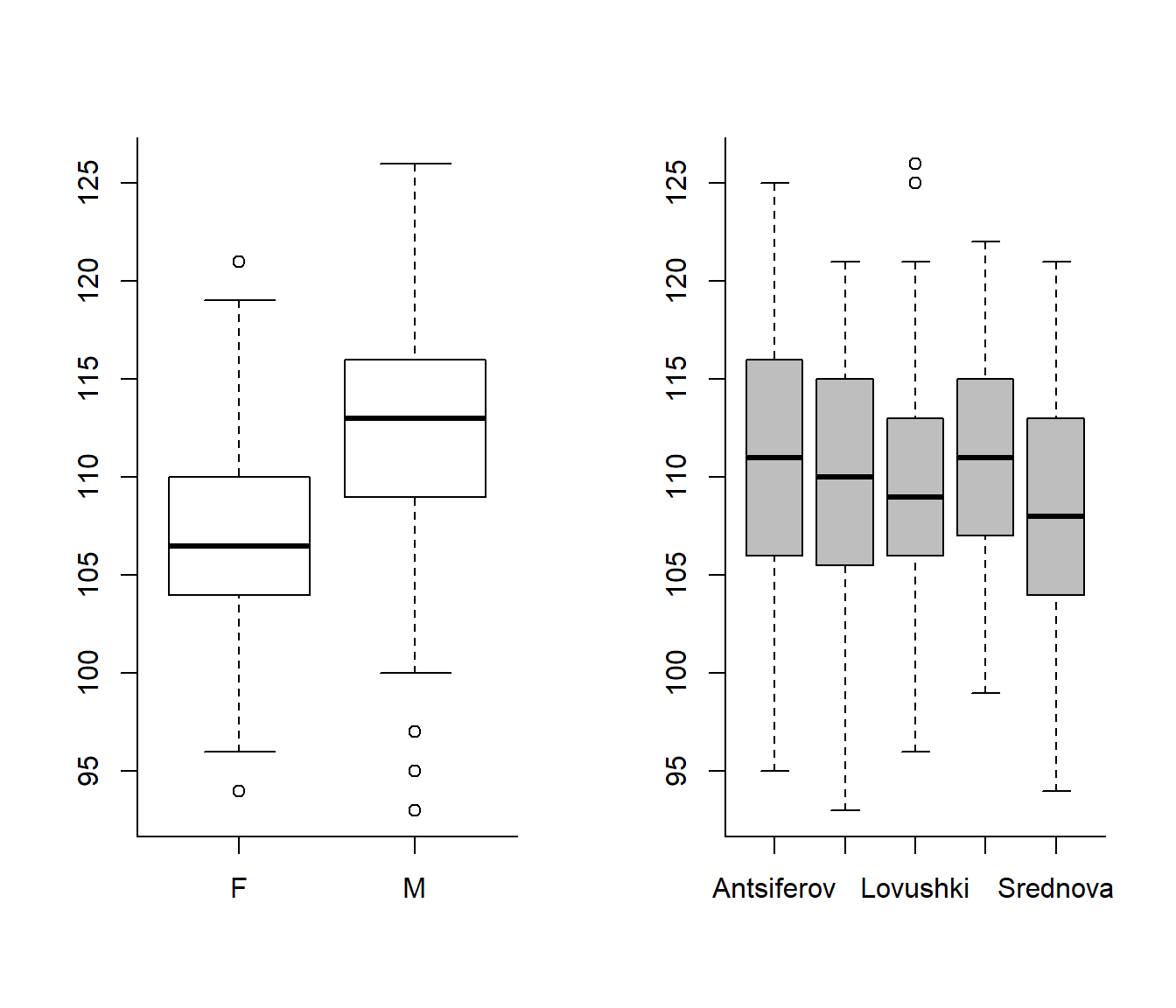
Note: the “+” notation:
boxplot(Length ~ Sex + Island, col="grey")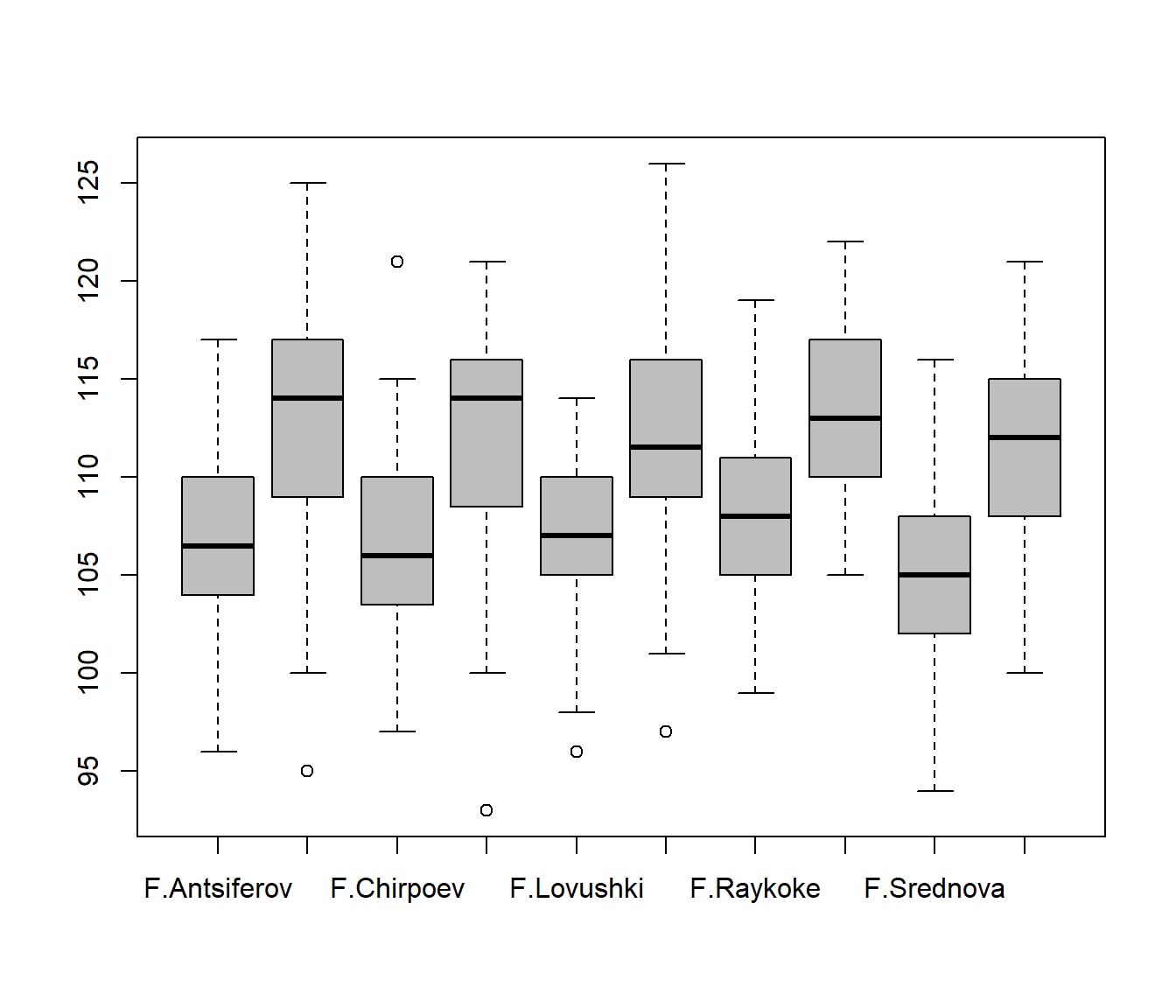
Also: “" does the same thing as “+” (e.g. boxplot(Length ~ Sex * Island)). The ~ notation is a very R specific way of defining models, with response variables to the left and explanatory variables to the right. For a box plot + and are equivalent. Their differences will become clear when we fit linear models with multiple interactions.
Labeling, and adding a legend:
  boxplot(Length ~ Sex * Island, col=2:3, xaxt="n")
  axis(1, at=1:5 * 2 - .5, levels(Island), cex.axis=1.25)
  legend("topright", fill=2:3, legend=levels(Sex), cex=1.5)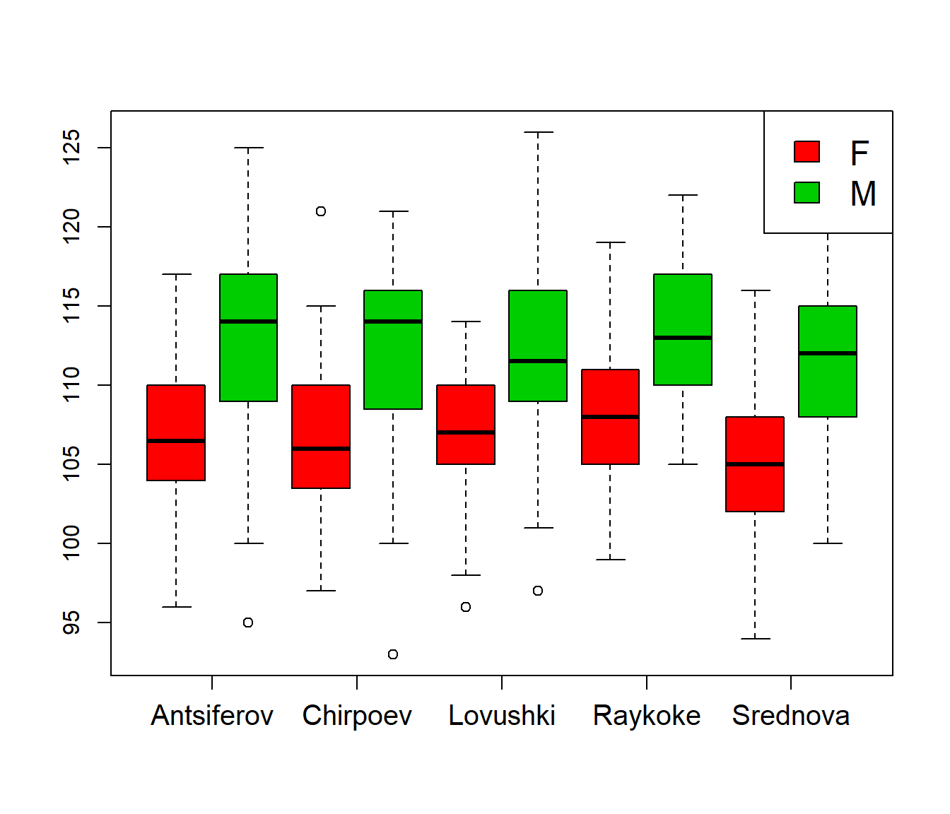
Tweaking locations, and adding transparency:
  boxplot(Length ~ Sex * Island, col=rgb(c(1,0),c(0,1),0,.5),
          xaxt="n", at=rep(1:5*2, each=2) + c(-.3,.3),
          ylab="Length (cm)", cex.lab=1.5)
  axis(1, at=1:5 * 2, levels(Island), cex.axis=1.25)
  legend("topright", fill=rgb(c(1,0),c(0,1),0,.5), legend=levels(Sex), cex=1.5)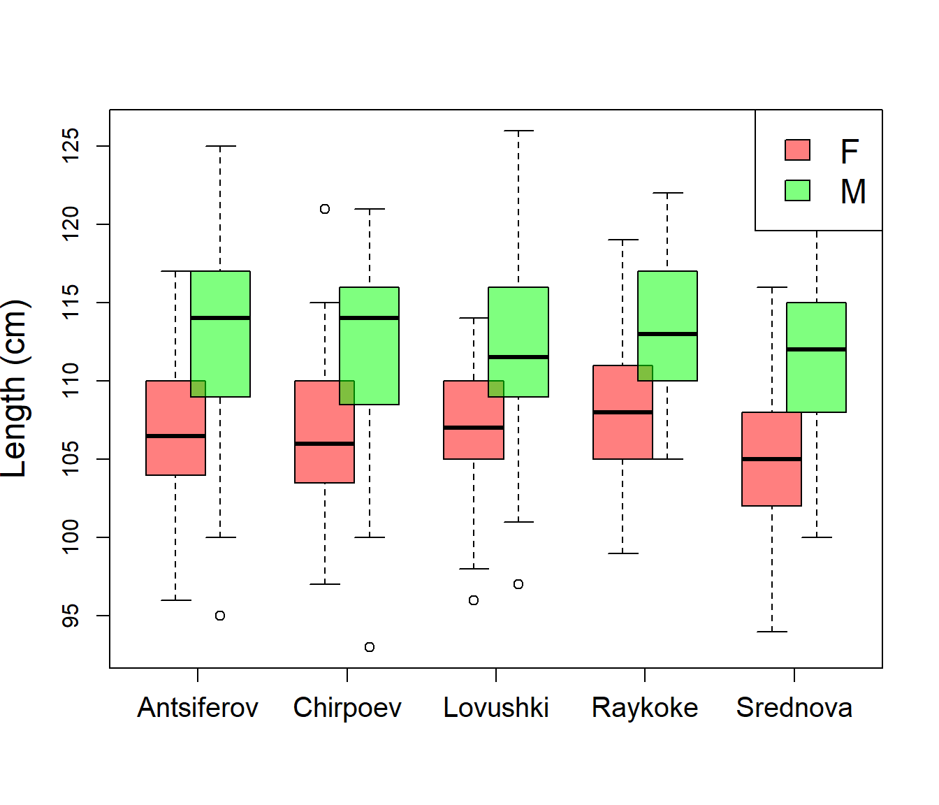
Compare with boxplot(Length ~ Island * Sex, col="grey"). What’s the difference?
Note, that you do not have to “extracted” the vectors for boxplots to work, you can just pass the data:
boxplot(Length ~ Sex * Island, data=Sealion, col="grey")
EXERCISE 2: GDP against Continents
Summarize, with quartiles, GDP with respect to continental region in CountryData.csv.
A basic box-plot of GDP by global region.
C <- read.csv("../_data/CountryData.csv")
myquantile <- function(x) quantile(x, na.rm=TRUE)
aggregate(C$GDP, list(C$Continent), myquantile)
## Group.1 x.0% x.25% x.50% x.75% x.100%
## 1 Africa 329.00 1026.50 1679.50 5065.50 23308.00
## 2 Asia 909.00 3119.25 6286.00 25852.00 88222.00
## 3 Europe 3092.00 12015.00 22195.00 35059.00 81466.00
## 4 North America 1163.00 7895.00 12561.00 14852.50 39171.00
## 5 Oceania 2307.00 4481.00 5799.00 27130.00 46860.00
## 6 South America 4604.00 7629.75 9475.50 12620.75 15901.00boxplot(GDP~Continent, data=C)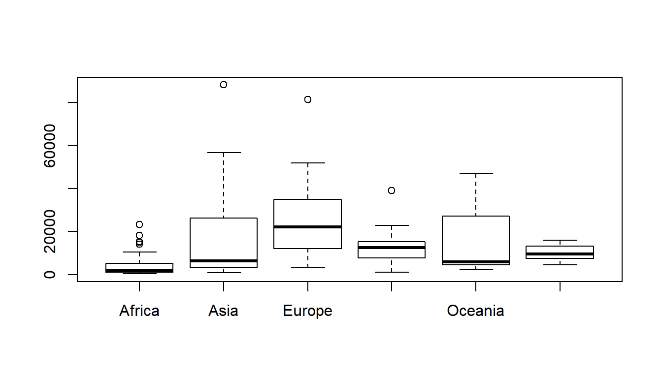
Making the width of the boxes proportional to sample size, and adding text labels (note the use of paste())
boxplot(GDP~Continent, data=C, varwidth=TRUE, col="grey")
text(1:6, 80000, paste("n =", tapply(C$GDP, C$Continent, length)), cex=1.5)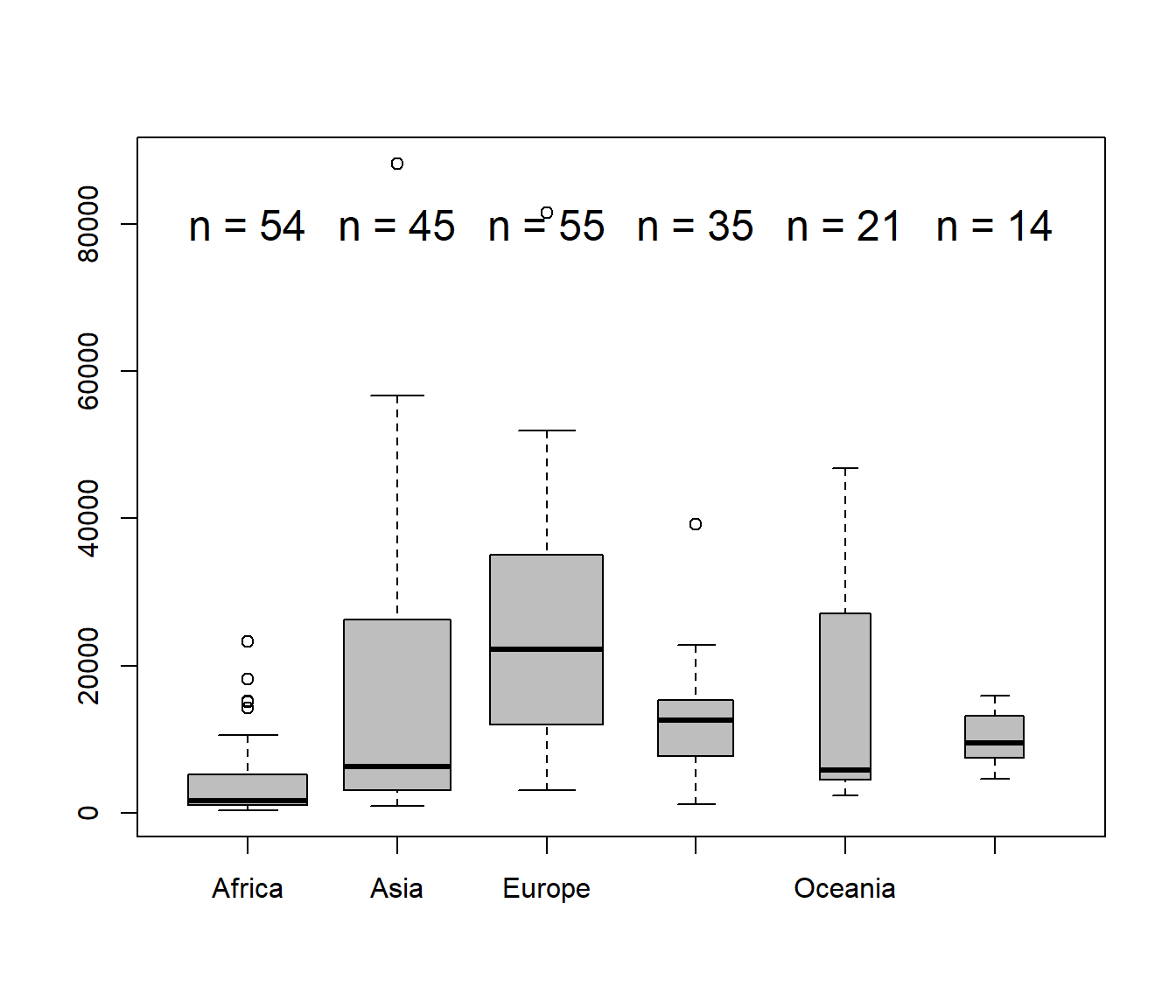
Multiple layers of information
The following code incrementally builds a scatter plot with several layers of quantitative and categorical information.
plot(C$GDP, C$Literacy)
plot(C$GDP, C$Literacy, log="x")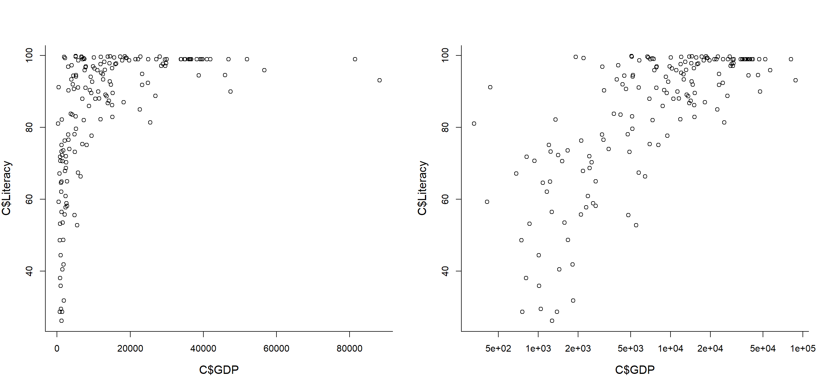
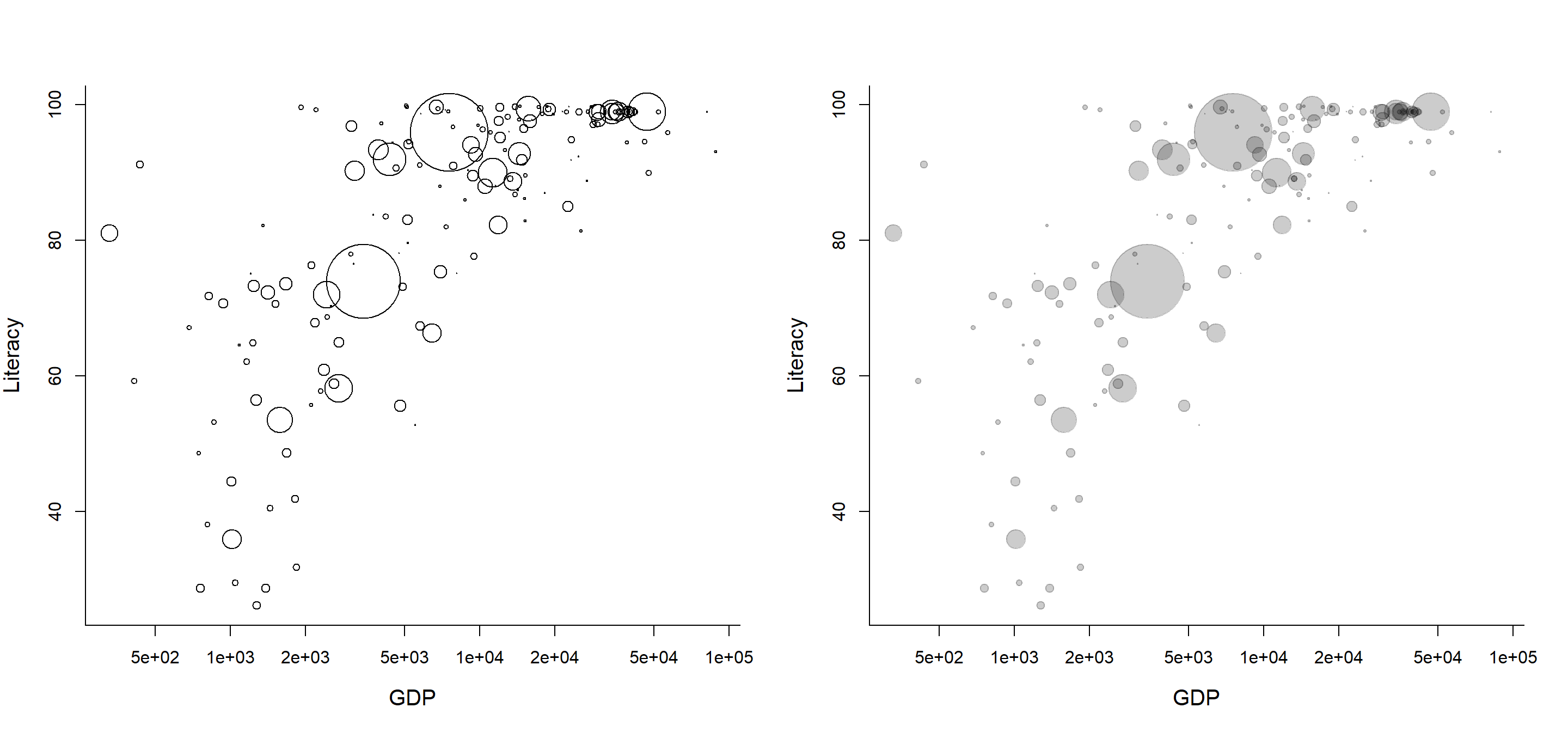
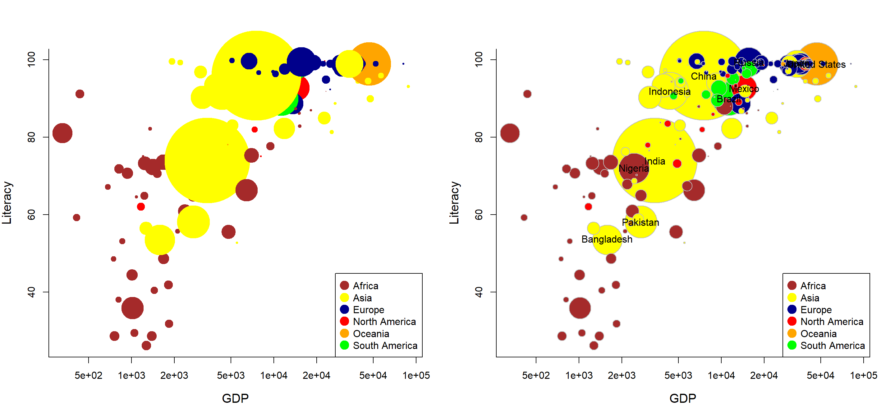
Make the circle areas proportional to population (note the “sqrt”), and the point character transparent:
with(C,
plot(GDP, Literacy, log="x",
     cex=sqrt(Population/max(Population, na.rm=TRUE))*10)
)

with(C,
    plot(GDP, Literacy, log="x",
     cex=sqrt(Population/max(Population, na.rm=TRUE))*10,
     pch=19, col=rgb(0,0,0,.2))
)
Color code the continents, reorder the data by decreasing population size, and, finally, label the largest countries:
# define a set of colors.  `alpha` is transparency.
cols <- c("brown","yellow","darkblue","red","orange","green")

with(C, {
    plot(GDP, Literacy, log="x",
             cex=sqrt(Population/max(Population, na.rm=TRUE))*20,
             pch=19, col=cols[match(Continent, levels(Continent))])
    legend("bottomright", legend=levels(Continent), col=cols, pch=19, pt.cex=2)
})

C <- C[order(C$Population, decreasing=TRUE),]
with(C, {
    plot(GDP, Literacy, log="x",
             cex=sqrt(Population/max(Population, na.rm=TRUE))*20,
             pch=21,
             col="grey",
             bg = cols[match(Continent, levels(Continent))])
    text(GDP[Population > 1e8],
             jitter(Literacy[Population > 1e8]),
             Country[Population > 1e8])
    legend("bottomright", legend=levels(Continent), col=cols, pch=19, pt.cex=2)
})
Note: there is a much “trendier” way to create graphics in R called ggplot, where the gg stands for “grammar of graphics”. As as example, to recreate something like the figure above you could use the following somewhat more compact (but - possibly - strange-looking) code:
require(ggplot2);  require(ggthemes)
ggplot(C, aes(x = GDP, y = Literacy, size = Population, color = Continent)) +
geom_point(alpha = 0.5) + scale_x_log10() + theme_few()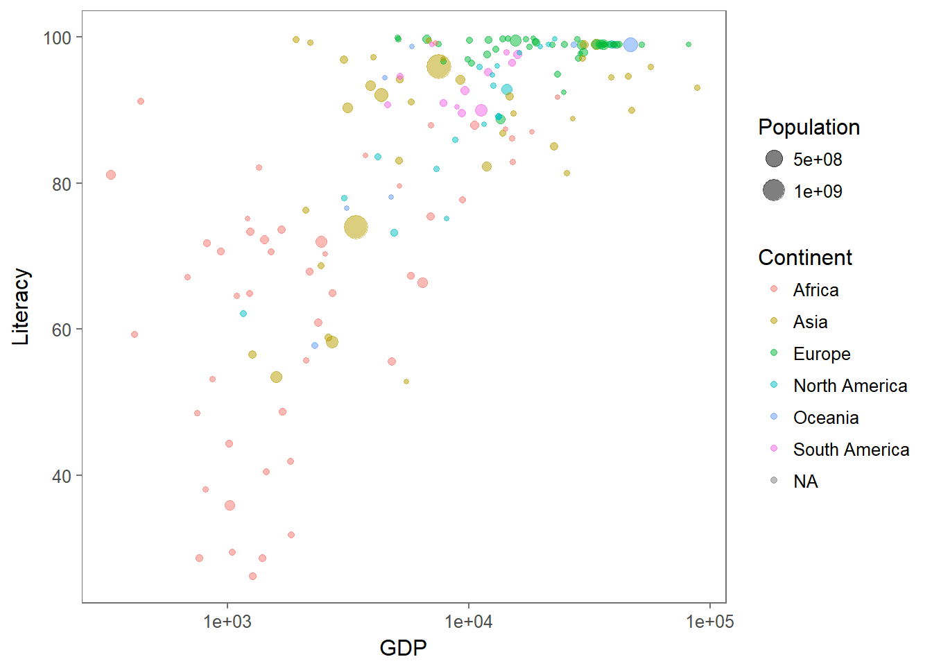
There are some objective advantages and disadvantages to base graphics and ggplot-ing. Personally, I find ggplots to be extremely useful for exploratory analysis of complex data, but have only every used base plotting to make figures for publications.
If there is strong demand, we may spend some time learning how to use ggplot.