Fitting Multiple Migrations
Elie Gurarie
2017-02-24
The key functions
You need to install the marcher package, which anyone can now do directly from GitHub.
require(devtools)
install_github("EliGurarie/marcher")
And loaded:
require(marcher)Key functions are posted here, which you can download or copy/paste:
source("./code/multimigration.r")or source directly off the web:
source("https://terpconnect.umd.edu/~egurarie/research/ABoVE/metamigration/code/multimigration.r")The functions are:
fitMultiMigration()- fittingplotMultimigrationFit()- plottingfinddate()- mini-helper function
Also:
Work flow for sample moose
These are daily averaged moose locations (see other file):
load("./data/moose_daily.robj")
head(moose.daily)
## id day day.date x y lon lat
## 1 20A019 292 2011-10-20 12:00:00 486821.5 7077002 -147.2677 63.82016
## 2 20A019 293 2011-10-21 12:00:00 484069.6 7076186 -147.3235 63.81272
## 3 20A019 294 2011-10-22 12:00:00 481531.5 7074471 -147.3749 63.79720
## 4 20A019 295 2011-10-23 12:00:00 481989.1 7074286 -147.3656 63.79557
## 5 20A019 296 2011-10-24 12:00:00 482329.2 7073795 -147.3586 63.79118
## 6 20A019 297 2011-10-25 12:00:00 482286.3 7076284 -147.3598 63.81352
## time elevation
## 1 2011-10-20 21:51:22 1346
## 2 2011-10-21 11:40:53 1373
## 3 2011-10-22 10:24:46 1123
## 4 2011-10-23 11:20:43 1150
## 5 2011-10-24 11:10:50 1288
## 6 2011-10-25 11:01:18 1144To perform the analysis you need data that have a day column (numeric, not POSIX), a POSIX time column, and x and y.
Moose C52
We’ll start with moose C52:
me <- subset(moose.daily, id == "C52")
with(me, scan.track(time = time, x = x, y = y))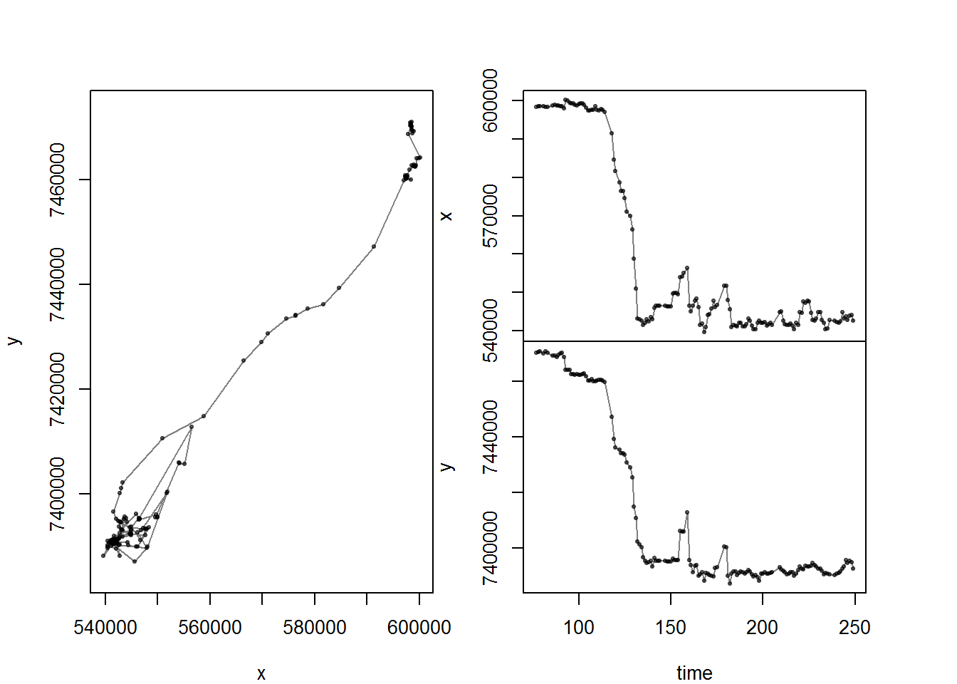
Lots of great migrations here. In fact, 9 in total (excluding the little foraging trip in 2011). The analysis will pick out single migrations (one at a time), and for each migration you need to pick the beggining and end of a “span”. For example, the first 250 days:
with(subset(me, day < 250), scan.track(time = day, x = x, y = y))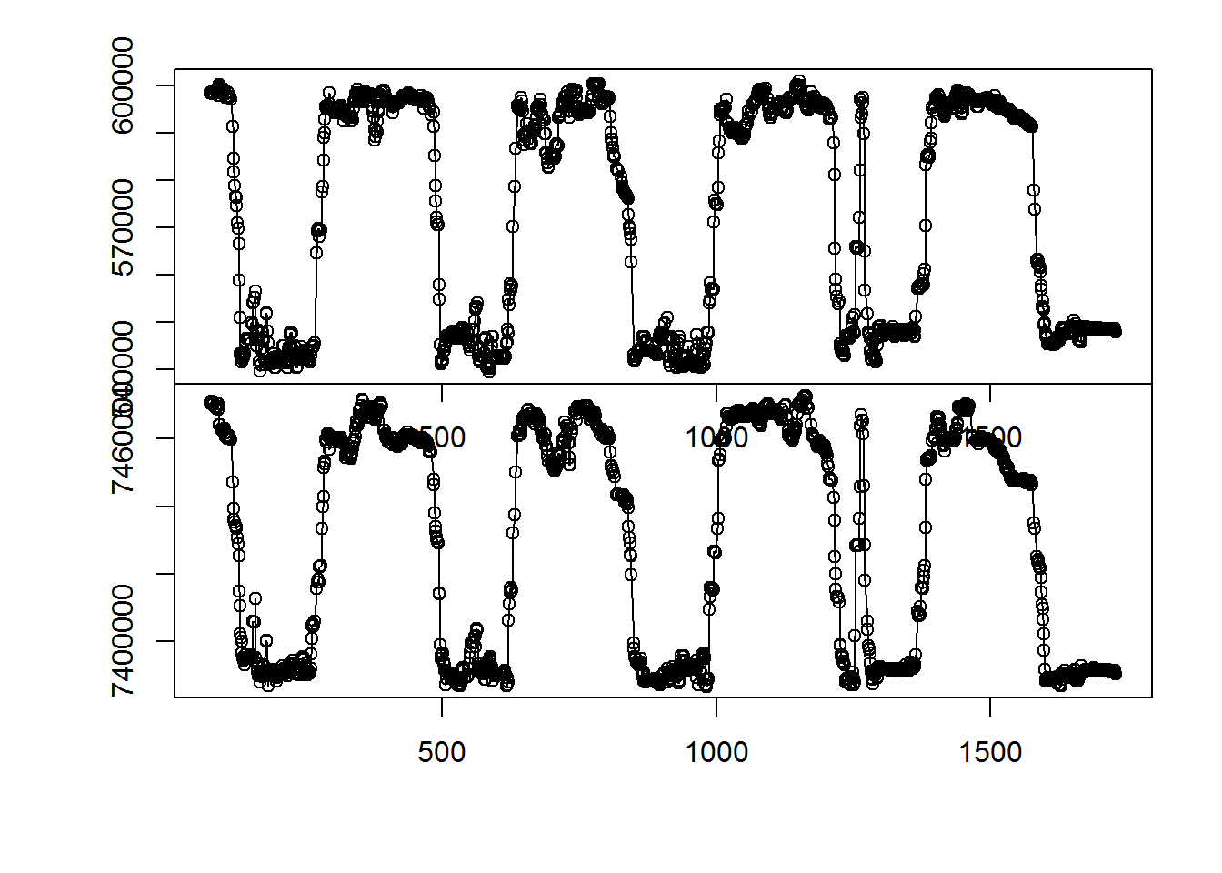
The key function (in marcher) is estimate.shift, which looks something like this:
myfit <- with(subset(me, day < 250), estimate.shift(T = day, X = x/1000, Y = y/1000, model = "WN"))
myfit
## Range shift estimation:
##
## 154 observations over time range 77 to 249.
## 2 ranges (one shift) fitted using the AR method.
##
## Initial shift parameters obtained from `quickfit`:
## t1 dt x1 y1 x2 y2
## 125.5 5.0 594.4 7459.0 544.7 7394.0
## The fitted ranging model is WN.
##
## Parameter Estimates:
## p.hat CI.low CI.high
## A 254.07869 213.94917 294.20821
## t1 113.37042 113.28810 113.45274
## dt 22.72192 22.59411 22.84972
## x1 598.70180 598.47841 598.92519
## y1 7464.85548 7464.63209 7465.07887
## x2 544.19592 544.06346 544.32839
## y2 7393.03367 7392.90120 7393.16613
##
## log-likelihood: -836.8; AIC: 1688; degrees of freedom: 7plot(myfit)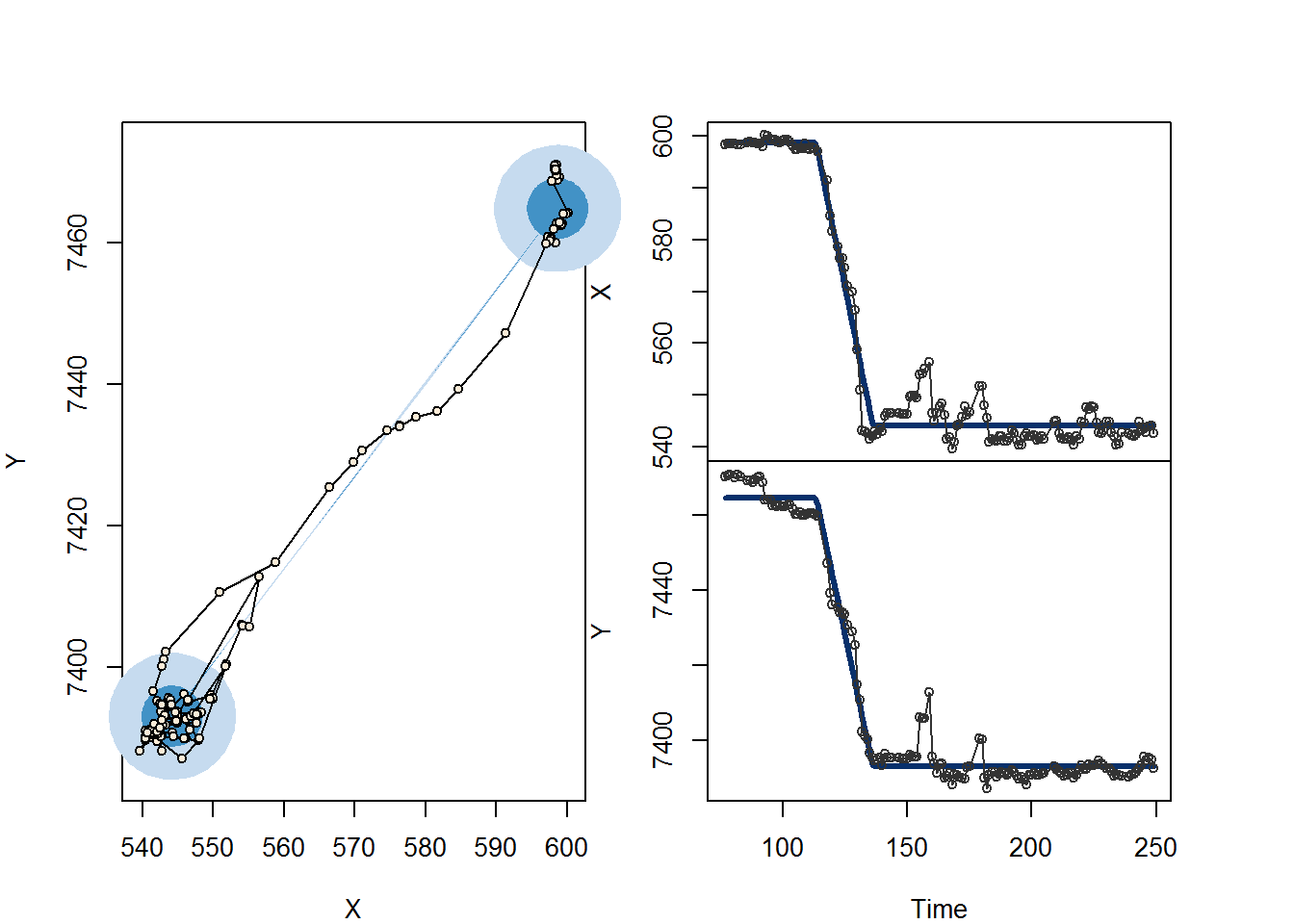
All the estimates are summarized in the table above, and the plot is a handy visualization of the single shift.
In order to fit multiple shifts conveniently, the fitMultiMigration function requires a dataset and two vectors: span1 and span2 which are the start and end times of each span. These should overlap. The best way to obtain them for an individual is to plot the times and x-y and use the locator function, i.e. make the following plots:
par(mfrow=c(2,1), mar = c(0,0,0,0), oma = c(5,5,2,2))
with(me, plot(day, x, type="o"))
with(me, plot(day, y, type="o"))
and run the following code:
span1 <- locator(9)$x
span2 <- locator(9)$x
clicking, respectively, on all of the beginnings and ends of the spans (in this case, 9 times each).
When I do this for this moose I get the following values:
span1 <- c(64, 140, 297, 507, 650, 855, 1021, 1293, 1406)
span2 <- c(254, 469, 602, 788, 964, 1191, 1247, 1566, 1741)
The analysis is performed in one line, which also generates a plot of the results for assessment purposes:
C52.migrations <- fitMultiMigration(me, span1, span2)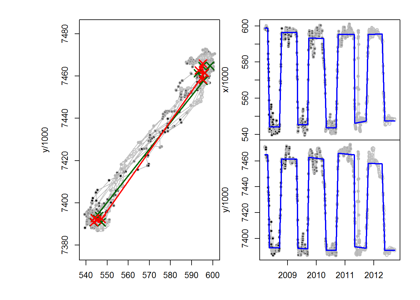
The lines show the fits. And the output is this table:
C52.migrations## id span1 span2 .id A t1 dt x1 y1
## 1 C52 64 254 M1 248.8101 2008-04-23 22.758666 598.6998 7464.857
## 2 C52 140 469 M2 228.6348 2008-09-19 28.243053 544.1313 7392.752
## 3 C52 297 602 M3 232.6837 2009-04-27 16.571449 596.2518 7461.443
## 4 C52 507 788 M4 393.3418 2009-09-11 18.645117 545.2609 7391.928
## 5 C52 650 964 M5 466.2665 2010-04-03 33.632958 593.0144 7461.380
## 6 C52 855 1191 M6 194.9563 2010-09-10 27.270951 543.8303 7390.880
## 7 C52 1021 1247 M7 382.9353 2011-04-26 9.687542 595.2003 7464.783
## 8 C52 1293 1566 M8 373.2287 2011-09-26 27.164840 547.4092 7392.387
## 9 C52 1406 1741 M9 278.7594 2012-04-15 36.932876 595.5801 7457.860
## x2 y2 yday1 month year season
## 1 544.1233 7392.908 114 4 2008 spring
## 2 596.2722 7461.623 263 9 2008 fall
## 3 545.3023 7392.419 117 4 2009 spring
## 4 593.3894 7462.733 254 9 2009 fall
## 5 543.6735 7390.819 93 4 2010 spring
## 6 595.3097 7465.965 253 9 2010 fall
## 7 546.1987 7393.690 116 4 2011 spring
## 8 595.2954 7458.344 269 9 2011 fall
## 9 547.4335 7390.737 106 4 2012 springWhich will be our ultimate source of analysis. Note that already we can do some prelinimary comparisons. For example:
boxplot(dt~season, data = C52.migrations)
It looks like the spring migrations are much more variable in duration than the fall migrations for this individualk … (maybe because the moose is more relaxed about getting to summering grounds?). A quick test:
(F.stat <- with(C52.migrations, var(dt[season == "spring"])/var(dt[season == "fall"])))## [1] 6.486625table(C52.migrations$season)##
## fall spring
## 4 51 - pf(F.stat, 4, 3)## [1] 0.078225Not quite significant p-value.
The other mooses
Anyways, here is the analysis for two other moose:
Moose C47
    me <- subset(moose.daily, id ==  "C47")
    with(me, scan.track(time = day.date, x = x, y = y))
Seven migrations. Following this interactive analysis:
    par(mfrow=c(2,1), mar = c(0,0,0,0), oma = c(5,5,2,2))
    with(me, plot(day, x, type="o"))
    with(me, plot(day, y, type="o"))
    span1 <- locator(7)$x
    span2 <- locator(7)$x
Yielding thiese numbers:
    span1 <- c(67, 196, 476, 550, 733, 912, 1053)
    span2 <- c(250, 519, 603, 713, 989, 1221, 1358)
And the analysis:
(C47.migrations <- fitMultiMigration(me, span1, span2))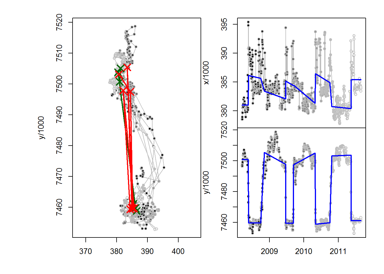
##    id span1 span2 .id         A         t1        dt       x1       y1
## 1 C47    67   250  M1 134.40747 2008-05-18  5.776598 381.0003 7500.774
## 2 C47   196   519  M2 359.76828 2008-09-30 37.451600 385.6342 7459.724
## 3 C47   476   603  M3  93.25786 2009-06-21  2.136330 382.0670 7497.878
## 4 C47   550   713  M4 113.12910 2009-09-10  2.819399 384.3801 7459.373
## 5 C47   733   989  M5 176.53361 2010-04-30  4.648745 381.3010 7505.082
## 6 C47   912  1221  M6 178.53234 2010-10-02 21.886982 384.9031 7459.871
## 7 C47  1053  1358  M7 127.34292 2011-05-15  2.313992 380.4014 7503.784
##         x2       y2 yday1 month year season
## 1 386.1057 7459.697   139     5 2008 spring
## 2 383.3913 7505.437   274     9 2008   fall
## 3 385.1281 7459.505   172     6 2009   fall
## 4 384.4567 7497.479   253     9 2009   fall
## 5 386.4469 7458.828   120     4 2010 spring
## 6 380.7109 7503.134   275    10 2010   fall
## 7 385.3980 7461.118   135     5 2011 spring
Moose 20A019
The last moose is the most challenging:
    me <- subset(moose.daily, id ==  "20A019")
    with(me, scan.track(time = day.date, x = x, y = y))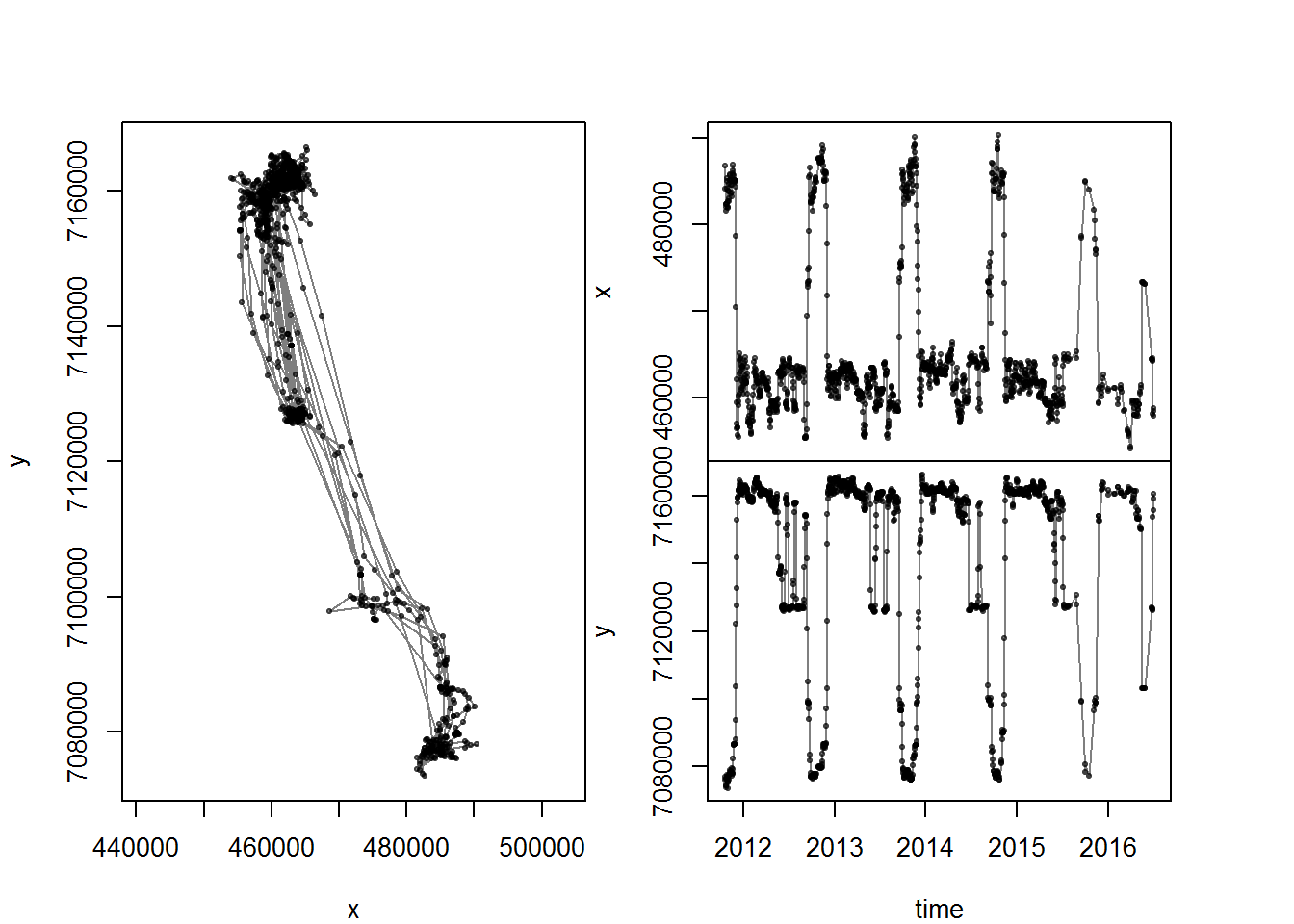
    span1 <- c(271, 359, 641, 717, 1008, 1085, 1370, 1429, 1725)
    span2 <- c(492, 682, 858, 1040, 1254, 1400, 1568, 1776, 1935)

    (M3.migrations <- fitMultiMigration(me, span1, span2))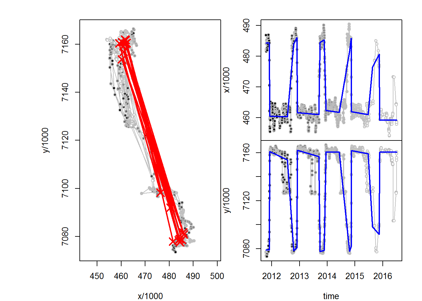
##       id span1 span2 .id          A         t1         dt       x1
## 1 20A019   271   492  M1  119.31381 2011-11-29   8.233002 484.2796
## 2 20A019   359   682  M2 1793.31181 2012-07-27  80.334303 460.3510
## 3 20A019   641   858  M3  102.63286 2012-11-28   5.841290 485.9900
## 4 20A019   717  1040  M4 1159.73486 2013-09-10  17.910748 461.0347
## 5 20A019  1008  1254  M5  129.48527 2013-11-22  21.757381 485.2351
## 6 20A019  1085  1400  M6  675.91794 2014-06-08 134.398430 461.6977
## 7 20A019  1370  1568  M7   91.98135 2014-11-10   5.310055 485.7310
## 8 20A019  1429  1776  M8  541.56335 2015-06-23  56.484336 461.0037
## 9 20A019  1725  1935  M9  290.26238 2015-11-14   8.225519 480.5575
##         y1       x2       y2 yday1 month year season
## 1 7078.966 460.4883 7160.867   333    11 2011   fall
## 2 7153.773 483.9015 7078.444   209     7 2012   fall
## 3 7080.813 461.6043 7162.002   333    11 2012   fall
## 4 7156.841 484.4153 7077.650   253     9 2013   fall
## 5 7078.669 462.3199 7160.547   326    11 2013   fall
## 6 7160.327 481.6532 7077.916   159     6 2014   fall
## 7 7081.730 461.9381 7161.768   314    11 2014   fall
## 8 7159.195 476.3965 7098.272   174     6 2015   fall
## 9 7091.990 459.2002 7160.415   318    11 2015   fall
Note that the “winter” periods for this moose are so short (usuall just a few months) that the “spring” migration actually occurs in November, which needs to be fixed “by hand”. Also, there are some strong stopover behaviors which are not accounted for (though there tools for that in marcher).
M3.migrations$season[M3.migrations$month == 11] <- "spring"Mini-preliminary joint analysis of migration durations
moose.migrations <- rbind(C52.migrations, C47.migrations, M3.migrations)

boxplot(dt ~ season*as.character(id), data = moose.migrations, col = 2:3)
A quick ANOVA:
anova(lm(dt~id+season, data = moose.migrations))## Analysis of Variance Table
##
## Response: dt
## Df Sum Sq Mean Sq F value Pr(>F)
## id 2 2798.9 1399.5 2.1941 0.13635
## season 1 4266.7 4266.7 6.6895 0.01722 *
## Residuals 21 13394.4 637.8
## ---
## Signif. codes: 0 '***' 0.001 '**' 0.01 '*' 0.05 '.' 0.1 ' ' 1A weak possible effect of season? In what direction?
summary(lm(dt~id+season, data = moose.migrations))##
## Call:
## lm(formula = dt ~ id + season, data = moose.migrations)
##
## Residuals:
## Min 1Q Median 3Q Max
## -34.323 -17.687 -3.160 9.812 82.165
##
## Coefficients:
## Estimate Std. Error t value Pr(>|t|)
## (Intercept) 52.23 10.14 5.151 4.2e-05 ***
## idC47 -29.95 12.79 -2.341 0.0292 *
## idC52 -13.07 11.91 -1.097 0.2849
## seasonspring -26.32 10.18 -2.586 0.0172 *
## ---
## Signif. codes: 0 '***' 0.001 '**' 0.01 '*' 0.05 '.' 0.1 ' ' 1
##
## Residual standard error: 25.26 on 21 degrees of freedom
## Multiple R-squared: 0.3453, Adjusted R-squared: 0.2518
## F-statistic: 3.693 on 3 and 21 DF, p-value: 0.02803Very small sample size, but possibly (in fact) a longer fall migration than spring migration. With a WHOLE BUNCH of moose, this (and more interesting) analyses can get more interesting very quickly.