Annotating data with elevations and NDVI
Elie Gurarie
2017-02-24
Load useful data manipulation / visualization packages:
pcks <- c("plyr", "ggplot2", "ggmap", "ggthemes", "magrittr", "lubridate", "scales")
a <- lapply(pcks, require, character.only = TRUE, quietly = TRUE)
Plotting Moose Migrations
Some loaded moose data. Recall, this was made in Part I, and can be easily recreated using the processMovedata() function.
load(file = "./data/moose_daily.robj")
head(moose.daily)
## id day day.date x y lon lat
## 1 20A019 292 2011-10-20 12:00:00 486821.5 7077002 -147.2677 63.82016
## 2 20A019 293 2011-10-21 12:00:00 484069.6 7076186 -147.3235 63.81272
## 3 20A019 294 2011-10-22 12:00:00 481531.5 7074471 -147.3749 63.79720
## 4 20A019 295 2011-10-23 12:00:00 481989.1 7074286 -147.3656 63.79557
## 5 20A019 296 2011-10-24 12:00:00 482329.2 7073795 -147.3586 63.79118
## 6 20A019 297 2011-10-25 12:00:00 482286.3 7076284 -147.3598 63.81352
## time elevation
## 1 2011-10-20 21:51:22 1346
## 2 2011-10-21 11:40:53 1373
## 3 2011-10-22 10:24:46 1123
## 4 2011-10-23 11:20:43 1150
## 5 2011-10-24 11:10:50 1288
## 6 2011-10-25 11:01:18 1144As you recall, there are three in alaska, and one way far south in Canada:
require(mapdata)
map("worldHires", xlim = range(moose.daily$lon) + c(-5,5), ylim = range(moose.daily$lat) + c(-5,5), col="grey"); box()
ddply(moose.daily, "id", function(df) with(df, lines(lon, lat, col=as.numeric(id[1]))))
## data frame with 0 columns and 0 rowslegend("bottomleft", col=1:4, legend = levels(moose.daily$id), lty=1, cex = 0.5, bty="n")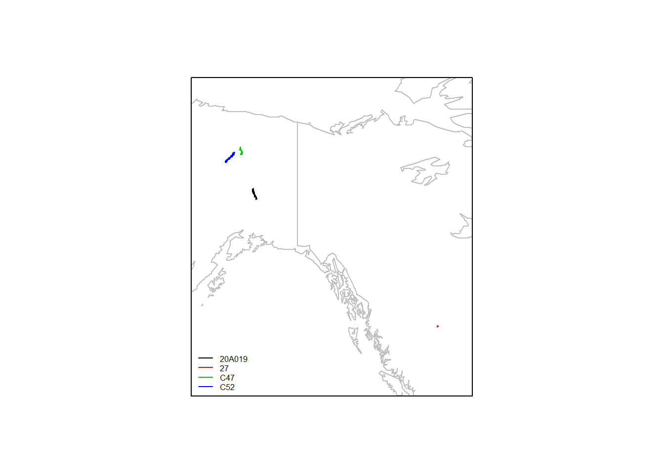
Annotating elevations
The new elevatr package allows you to easily access the Mapzen terrain service.
Warning: this announcements just showed up on their website:
Announcement: API keys required to use Mapzen services: Effective March 2017, API keys are required when you use Mapzen services. This ensures your users have good experiences with your apps.
So there’s a good chance this code will only work for the next week without some tweaks.
An example using one of the mooses:
require(elevatr)
me <- subset(moose.daily, id == "C52")
proj <- "+proj=longlat +ellps=WGS84 +datum=WGS84 +no_defs"
m2 <- mutate(me, elevation = get_elev_point(data.frame(x = lon, y = lat), prj = proj, src = "mapzen", api_key = "mapzen-91tYY4s"))
m2$elevation <- as.numeric(m2$elevation@data[,1])
This function lets you visualize the migration in three dimensions
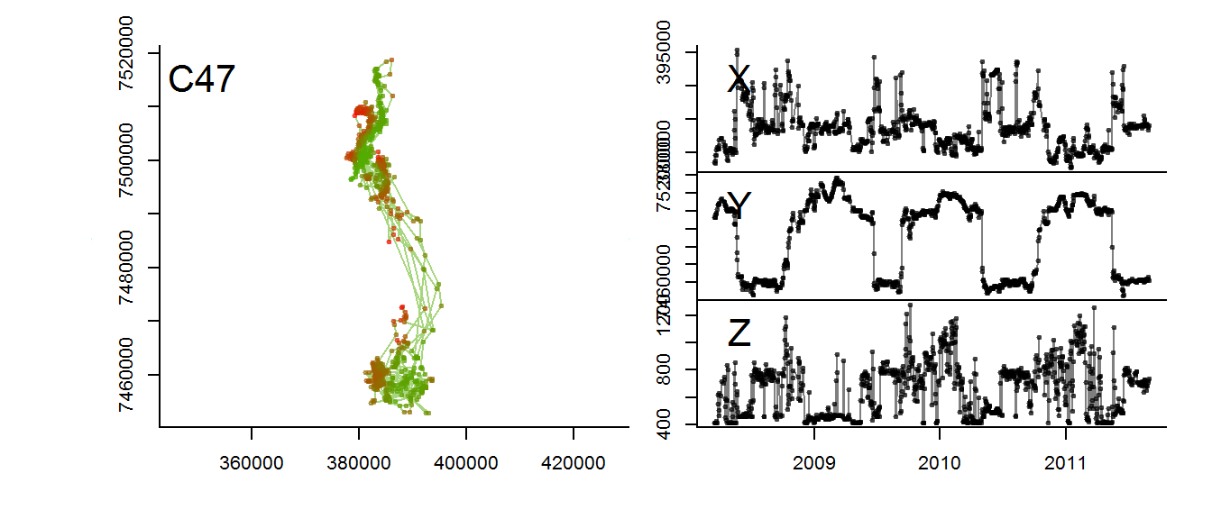
scan.track.z <- function(time, x, y, z, title = "",...)
{
  par(mar = c(0,3,0,0), oma = c(4,4,2,2))
  layout(rbind(c(1,2), c(1,3), c(1,4)))

  MakeLetter <- function(a, where="topleft", cex=2)
     legend(where, pt.cex=0, bty="n", title=a, cex=cex, legend=NA)

  plot(x,y,asp=1, type="o", pch=19, col=rgb(z/max(z),(1-z/(max(z))),0,.5), cex=0.5, ...); MakeLetter(title)
  plot(time,x, type="o", pch=19, col=rgb(0,0,0,.5), xaxt="n", xlab="", cex=0.5, ...); MakeLetter("X")
  plot(time,y, type="o", pch=19, col=rgb(0,0,0,.5), xaxt="n", xlab="", cex=0.5, ...); MakeLetter("Y")
  plot(time,z, type="o", pch=19, col=rgb(0,0,0,.5), cex=0.5, ...); MakeLetter("Z")
}
Illustrate:
with(m2, scan.track.z(time = time, x=x, y=y, z = elevation))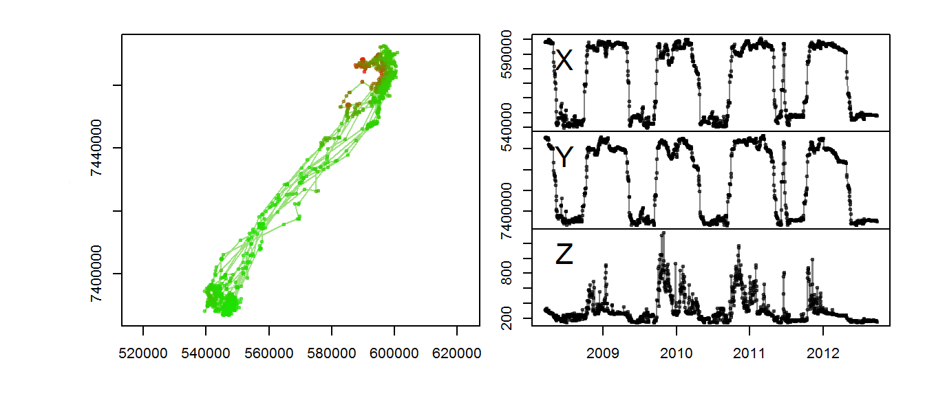
The altitudinal signal for this moose is actually not very clear.
In this line, we obtain elevations for all moose locations and save the file (for later analysis).
moose.daily <- mutate(moose.daily, elevation = get_elev_point(data.frame(x = lon, y = lat), prj = proj, src = "mapzen", api_key = "mapzen-91tYY4s")@data[,1])
save(moose.daily, file = "./data/moose_daily.robj")
Finally, the other mooses:
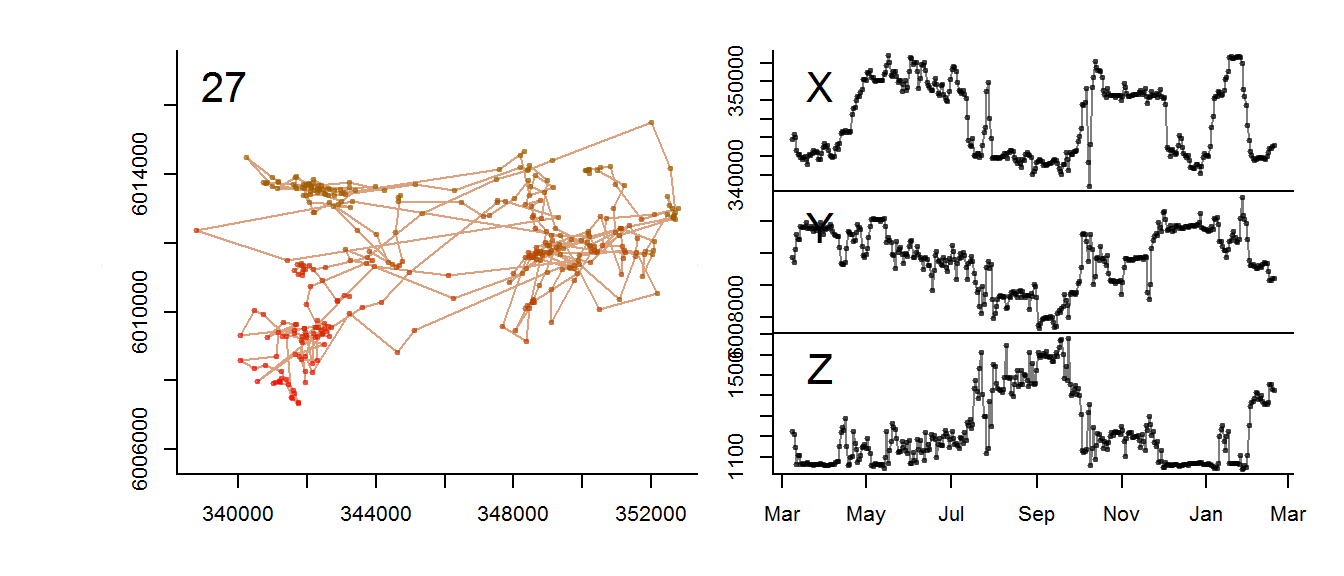
for(myid in levels(moose.daily$id)[1:3])
with(subset(moose.daily, id == myid),
     scan.track.z(time = time, x=x, y=y, z = elevation, title = myid))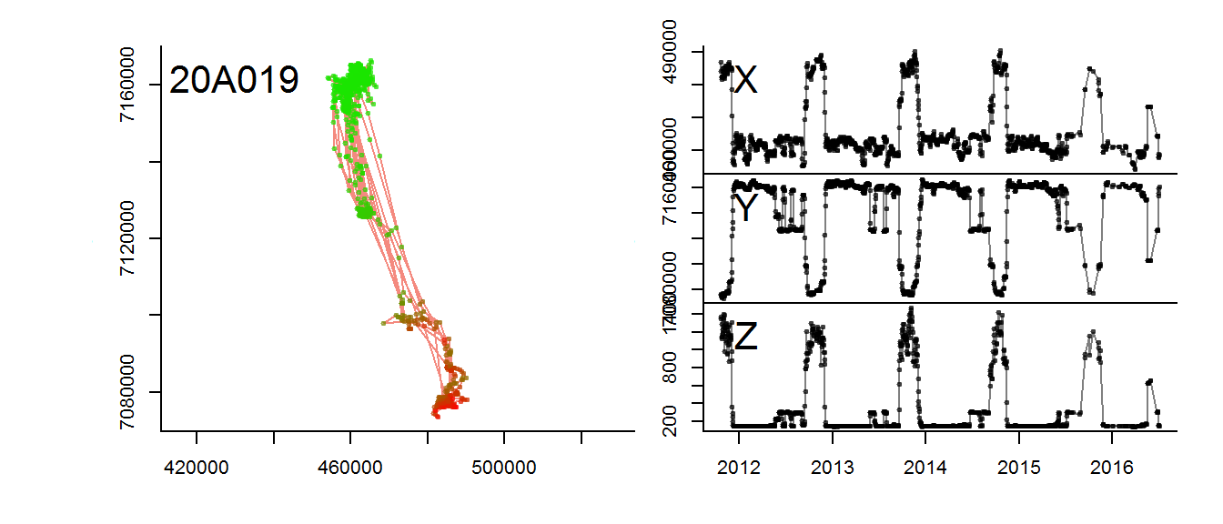
Annotating with MODIS data
An important warning … the CRAN MODISTools does NOT work because of outdated / unsupported dependencies (see this thread: https://groups.google.com/forum/#!topic/predicts_project/FctDowcYgx0). You have to install if from GIT-hub:
library(devtools)
install_git("http://github.com/seantuck12/MODISTools")
It might ask you to install a bunch of dependent packages (like XML - it did for me).
Load the package.
require(MODISTools)I don’t know too much about MODIS products, e.g. what product and band is best. But for now we’ll just get the NDVI value for “MOD13Q1” at just two locations - one in the summer range and one at the winter range.
summer <- c(-152, 66.65)
winter <- c(-150.75, 67.3)
points <- rbind(summer, winter)

with(subset(moose.daily, id == "C52"), plot(lon, lat))
points(points, col=2, pch = 4, cex=3, lwd=2)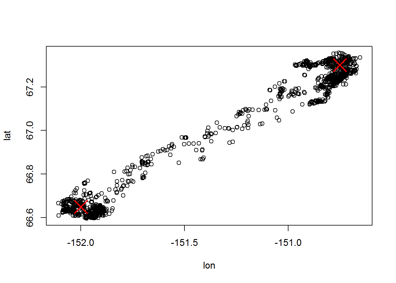
The available bands are:
product <- "MOD13Q1"
GetBands(product)
## [1] "250m_16_days_blue_reflectance"
## [2] "250m_16_days_MIR_reflectance"
## [3] "250m_16_days_NIR_reflectance"
## [4] "250m_16_days_pixel_reliability"
## [5] "250m_16_days_red_reflectance"
## [6] "250m_16_days_relative_azimuth_angle"
## [7] "250m_16_days_sun_zenith_angle"
## [8] "250m_16_days_view_zenith_angle"
## [9] "250m_16_days_VI_Quality"
## [10] "250m_16_days_NDVI"
## [11] "250m_16_days_EVI"
## [12] "250m_16_days_composite_day_of_the_year"Let’s go with NDVI
band <- c("250m_16_days_NDVI")
pixel <- c(0,0)
You have to specify the x/y/time range of the desired data:
period <- data.frame(lat=points[,2], long=points[,1], start.date=2008, end.date=2012, id=1)The key function (and this takes a while) is MODISSubsets. This will download a file and save it in the specified SaveDir. This takes a while … multiple minutes on my computer.
MODISSubsets(LoadDat = period, FileSep = "", Products = product, Bands = band, Size = pixel, SaveDir = "./data", StartDate = TRUE)Files downloaded will be written to ./data. Found 2 unique time-series to download. Getting subset for location 1 of 2… Getting subset for location 2 of 2… Full subset download complete. Writing the subset download file… Done! Check the subset download file for correct subset information and download messages.
This function downloaded two files: Lat66.65000Lon-152.00000Start2008-01-01End2012-12-31___MOD13Q1.asc and Lat67.30000Lon-150.75000Start2008-01-01End2012-12-31___MOD13Q1.asc.
These are difficult files to parse, but there are some functions that simplify their analysis. MODISTimeSeries extracts the time series from all the available .asc files in the directory as a matrix:
mooseNDVI.ts <- MODISTimeSeries(Dir = "./data", Band = band, Simplify = TRUE)
head(mooseNDVI.ts)
## Lat66.65Lon-152Samp1Line1_pixel1
## A2008001 -3000
## A2008017 -1988
## A2008033 976
## A2008049 831
## A2008065 466
## A2008081 792
## Lat67.3Lon-150.75Samp1Line1_pixel1
## A2008001 -3000
## A2008017 -570
## A2008033 -45
## A2008049 321
## A2008065 276
## A2008081 376colnames(mooseNDVI.ts) <- c("ndvi.summer", "ndvi.winter")The row names of this matrix contain the date of the measurement, as the YEAR-DAYOFYEAR. This takes some manipulation to turn into a POSIX:
require(lubridate)
mooseNDVI.ts <- data.frame(mooseNDVI.ts, date = ymd(paste(substring(row.names(mooseNDVI.ts), 2,5), 1, 1)) +
  ddays(as.numeric(substring(row.names(mooseNDVI.ts), 6))))
Ok, now we can at least plot these NDVI bands underneath the migration of the moose:
with(subset(moose.daily, id == "C52"),
     plot(time, lat, type="o", xlim = range(mooseNDVI.ts$date), xlab = "", xaxt="n", ylab = "latitude", pch = 19, col = rgb(0,0,0,.3), cex = 0.8))

with(mooseNDVI.ts,{
    plot(date, ndvi.summer, type="o", pch = 19, col = 2, ylab = "MODIS NDVI")
    lines(date, ndvi.winter, type="o", pch = 19, col = 4)
})
legend("topleft", col = c(2,4), legend = c("summer range", "winter range"), pch = 19, lty = 1, cex=0.75)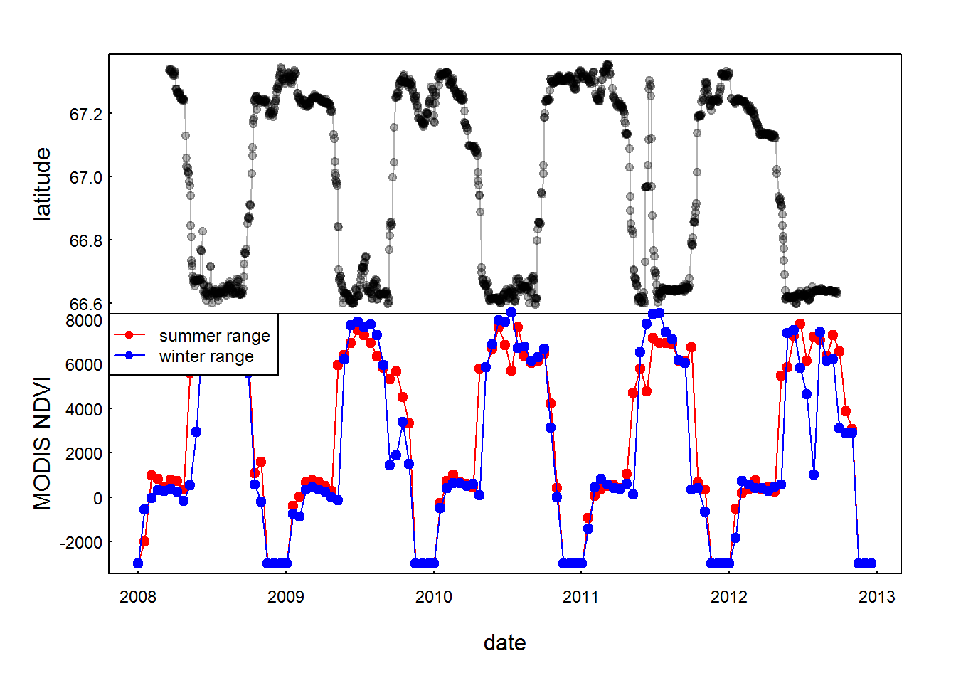
There’s not a lot of difference in the winter and summer ranges. Interesting that (superficially) it looks like the moose are initiating their winter migration before the plummeting in the NDVI actually happens.