Loading data from Movebank with R
Scott LaPoint (edited by Elie)
November 3, 2016
The following should help you directly access movebank.org via R, import movement data that you have permission to download, and convert these data into a data frame. I kept it brief and general deliberately. I use Windows, but I believe this will work on Linux and Mac as well. In the past, the RCurl package was necessary for some ssl issues, but I believe that is solved. Let me know if this is still an issue; I have/had some lines to deal with it.
## install.packages("move")
library(move)
Step 1: A Login Object
Create a movebank.org login object, using your username and password
## login <- movebankLogin(username="xxxx", password="xxxx")Step 2: Loading a study
If you wanted to import an entire movebank study (i.e., all individuals) run the following line. Remember to change the study name. This will only work on studies where you have permission to download the study.
ge <-getMovebankData(study="ABoVE: HawkWatch International Golden Eagles", login=login, removeDuplicatedTimestamps=T)Note, the ‘removeDuplicatedTimestamps=T’ will do as it says, which is not always the perfect solution, but for now it’s quick and dirty.
This should have loaded the golden eagle data:
head(ge)## location_error_text location_lat location_long timestamp
## 3749 <26 m 40.424 -114.271 2004-09-25 11:37:00
## 3750 150-349 m 41.905 -113.464 2004-12-05 23:40:48
## 3751 <150 m 41.906 -113.478 2004-12-06 00:19:49
## 3752 >1000 m 41.908 -113.404 2004-12-06 01:18:52
## 3753 >1000 m 41.893 -113.574 2004-12-06 01:23:52
## 3754 no estimate, < 3 msgs. 41.818 -113.478 2004-12-06 02:02:54
## argos_iq argos_lat1 argos_lat2 argos_lc argos_lon1 argos_lon2
## 3749 11 40.424 40.424 G -114.271 -114.271
## 3750 11 41.905 41.905 2 -113.464 -113.464
## 3751 11 41.906 41.906 3 -113.478 -113.478
## 3752 11 41.908 41.908 0 -113.404 -113.404
## 3753 11 41.893 41.893 0 -113.574 -113.574
## 3754 11 41.818 41.818 B -113.478 -113.478
## argos_nb_mes comments manually_marked_outlier sensor_type_id
## 3749 2 StartPoint 82798
## 3750 2 82798
## 3751 2 82798
## 3752 2 82798
## 3753 2 82798
## 3754 2 82798
## deployment_id event_id
## 3749 171299033 1604825587
## 3750 171299033 1604827509
## 3751 171299033 1604827510
## 3752 171299033 1604827511
## 3753 171299033 1604827512
## 3754 171299033 1604827513This is a “MoveStack” object, i.e. an S4 (formal class) with a bunch of “slots” containing information:
slotNames(ge)## [1] "trackId" "timestamps"
## [3] "idData" "sensor"
## [5] "data" "coords.nrs"
## [7] "coords" "bbox"
## [9] "proj4string" "trackIdUnUsedRecords"
## [11] "timestampsUnUsedRecords" "sensorUnUsedRecords"
## [13] "dataUnUsedRecords" "dateCreation"
## [15] "study" "citation"
## [17] "license"Here are the counts of observations per eagle:
table(ge@trackId)##
## X21166b X20948b X21259b X26353c X37300a X37301b X26353b X26401a X26400b
## 907 442 71 431 764 591 194 194 1214
## X37434a X37307a X37302a X21260c X18549b X26353d X26400a X20948a X21166c
## 801 1104 1346 3346 598 220 362 150 195
## X37301a X21168b X26359c X26359b X37305a X37306a X21260b X11515a X71527a
## 195 905 4302 145 1092 336 472 707 630
## X37303a X71526a X37304a X37433a X26401b X21839b
## 676 1221 1032 574 494 203Here is the bounding box:
ge@bbox## min max
## location_long -169.468 -37.046
## location_lat 20.009 69.974etc.
You can also select one animal/individual from a study as well:
goea21260c<-getMovebankData(study="ABoVE: HawkWatch International Golden Eagles", animalName="21260c", login=login, moveObject=TRUE)Some summary information about this eagle:
summary(goea21260c)## $X21260c
## TravDist MaxDist MinDist FarthDist AverDist SDDist SEDist
## 1 51381702 644386.3 0 3148.493 15360.75 48566.04 1169.914
##
## $X21260c
## Duration AverDur SDDur dupl multseason
## 1 26885.94 hours 8.037652 22.02393 FALSE FALSE
##
## $X21260c
## AverSpeed VarSpeed MaxSpeed
## 1 7.447866 904.2545 902.0186
##
## $X21260c
## AverAzimuth VarAzimuth SEAzimuth
## 1 126.2604 0.9718466 58.12135Note that the average speed is 7.4 (units unclear), but the maximum and variance are over 900! This suggests a lot of stopping and going.
Step 3. Mapping the data
S4 objects can be tricky to work with … for analysis R is much better suited to working with data frames and lists.
ge.df <- as.data.frame(ge)
str(ge.df)
## 'data.frame': 25914 obs. of 18 variables:
## $ location_error_text : Factor w/ 10 levels "<150 m","<26 m",..: 2 4 1 3 3 9 3 6 1 6 ...
## $ location_lat : num 40.4 41.9 41.9 41.9 41.9 ...
## $ location_long : num -114 -113 -113 -113 -114 ...
## $ timestamp : POSIXct, format: "2004-09-25 11:37:00" "2004-12-05 23:40:48" ...
## $ argos_iq : int 11 11 11 11 11 11 11 11 11 11 ...
## $ argos_lat1 : num 40.4 41.9 41.9 41.9 41.9 ...
## $ argos_lat2 : num 40.4 41.9 41.9 41.9 41.9 ...
## $ argos_lc : Factor w/ 8 levels "","0","1","2",..: 8 4 5 2 2 7 2 3 5 3 ...
## $ argos_lon1 : num -114 -113 -113 -113 -114 ...
## $ argos_lon2 : num -114 -113 -113 -113 -114 ...
## $ argos_nb_mes : int 2 2 2 2 2 2 2 2 2 2 ...
## $ comments : Factor w/ 2 levels "","StartPoint": 2 1 1 1 1 1 1 1 1 1 ...
## $ manually_marked_outlier: Factor w/ 2 levels "","true": 1 1 1 1 1 1 1 1 1 1 ...
## $ sensor_type_id : int 82798 82798 82798 82798 82798 82798 82798 82798 82798 82798 ...
## $ deployment_id : int 171299033 171299033 171299033 171299033 171299033 171299033 171299033 171299033 171299033 171299033 ...
## $ event_id : int 1604825587 1604827509 1604827510 1604827511 1604827512 1604827513 1604827514 1604827515 1604827516 1604827517 ...
## $ location_long.1 : num -114 -113 -113 -113 -114 ...
## $ location_lat.1 : num 40.4 41.9 41.9 41.9 41.9 ...Here’s a quick ggmap of all the eagles:
Generate “basemap”
basemap <- get_map(location = ge@bbox, maptype = "satellite")To make the plot look better, we need to convert the deployment_id to a factor:
ge.df$ID <- as.factor(ge.df$deployment_id)Plot all the individuals:
require(gplots)
ggmap(basemap) +
geom_point(data = ge.df, mapping = aes(x = location_long, y = location_lat, col=ID), alpha = 0.5, size=0.5) +
geom_path(data = ge.df, mapping = aes(x = location_long, y = location_lat, col = ID), alpha = 0.2) +
coord_map()+
scale_color_manual(values = rich.colors(length(unique(ge.df$ID)))) +
labs(x = "Longitude", y = "Latitude") + ggtitle("Golden Eagle locations") +
theme_few()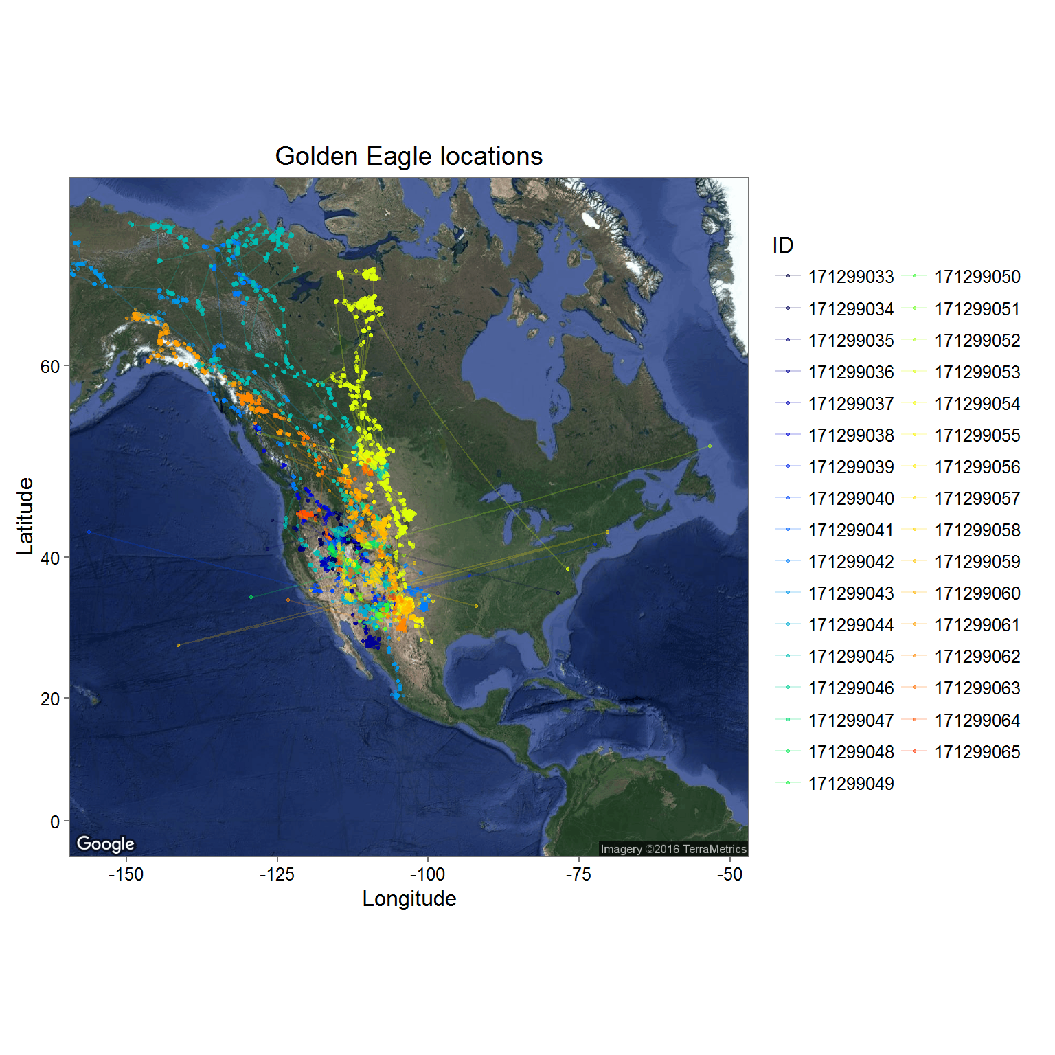
There are a few bells-and-whistles in this code to make it “prettier” to my (EG’s) eye that aren’t so important. But basically, you can see all the data at a glance, including some obviously wrong locations.