Most scientific
measurements involve the use of an instrument that actually
measures something else and converts it to the desired
measure. Examples are simple weight scales (which actually
measure the compression of a spring), thermometers (which
actually measure thermal expansion), pH meters (which
actually measure a voltage), and devices for measuring
hemoglobin in blood or CO2 in air (which actually measure the
intensity of a light beam). These instruments are
single-purpose, designed to measure one quantity, and
automatically convert what they actually measure into the
the desired quantity and display it directly. But to insure
accuracy, such instruments must be calibrated,
that is, used to measure one or more calibration standards
of known accuracy, such as a standard weight or a sample
that is carefully prepared to a known temperature, pH, or
sugar content. Most are pre-calibrated at the factory for
the measurement of a specific substance in a specific type
of sample.
Analytical
calibration. General-purpose
instrumental techniques that are used to measure the
quantity of many different chemical components in unknown
samples, such as the various kinds of spectroscopy,
chromatography, and electrochemistry, or combination
techniques like "GC-mass
spec", must also be calibrated, but because those
instruments can be used to measure a wide range of compounds
or elements, they must be calibrated by
the
user for
each substance and for each type of sample. Usually this is
accomplished by carefully preparing (or purchasing) one or
more "standard samples" of known concentration, such as
solution samples in a suitable solvent. Each standard is
inserted or injected into the instrument, and the resulting
instrument readings are plotted against the known
concentrations of the standards, using least-squares calculations to
compute the slope and
intercept, as
well as the standard deviation of the slope (sds)
and intercept (sdi).
Then the "unknowns" (that is, the samples whose
concentrations are to be determined) are measured by the
instrument and their signals are converted into
concentrations with the aid of the calibration curve. If the
calibration is linear, the sample concentration C of any
unknown is given by (A - intercept) /
slope,
where A is the measured signal (height or area) of that
unknown. The predicted standard deviation in the sample
concentration is C*SQRT((sdi/(A-intercept))^2+(sds/slope)^2)
by the rules for propagation of error.
All these calculations can be done in a spreadsheet, such as
CalibrationLinear.xls.
In some cases the thing measured can not be detected
directly but must undergo a chemical reaction that makes it
measurable; in that case the exact same reaction must be
carried out on all the standard solutions and unknown sample
solutions, as demonstrated
in
this animation (thanks to Cecilia Yu of Wellesley
College).
Various calibration methods are used to compensate for
problems such as random errors in standard preparation or
instrument readings, interferences,
drift, and non-linearity in the
relationship between concentration and instrument reading.
For example, the standard addition calibration
technique can be used to compensate for multiplicative
interferences. I have prepared a series of
"fill-in-the-blanks" spreadsheet
templates for various calibrations methods, with instructions,
as well as a series of spreadsheet-based
simulations of the error
propagation in widely-used analytical calibration
methods, including a step-by-step
exercise.
Calibration
and
signal processing.
Signal processing often intersects with calibration. For
example, if you use smoothing or filtering to reduce noise, or differentiation
to reduce the effect of
background, or measure peak
area
to reduce the effect of peak broadening, or use modulation to reduce the effect 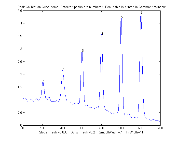 of low-frequency
drift, then you must use
the exact same signal processing for both the standard
samples and the unknowns, because the choice of signal
processing technique can have a big impact on the magnitude
and even on the units of
the resulting processed signal (as for example in the derivative technique and in
choosing between peak height and peak area).
of low-frequency
drift, then you must use
the exact same signal processing for both the standard
samples and the unknowns, because the choice of signal
processing technique can have a big impact on the magnitude
and even on the units of
the resulting processed signal (as for example in the derivative technique and in
choosing between peak height and peak area).
PeakCalibrationCurve.m
is an Matlab/Octave example of this. This script simulates
the calibration of a flow
injection system that produces signal peaks that are
related to an underlying concentration or amplitude ('amp').
In this example, six known standards are measured
sequentially, resulting in six separate peaks in the
observed signal. (We assume that the detector signal is
linearly proportional to the concentration at any instant).
To simulate a more realistic measurement, the script adds
four sources of "disturbance" to the observed signal:
a. noise - random white noise added to all the signal data points, controlled by the variable "Noise";
b. background - broad curved background of random amplitude, tilt, and curvature, controlled by "background";
c. broadening - exponential peak broadening that varies randomly from peak to peak, controlled by "broadening";
d. a final smoothing before the peaks are measured, controlled by "FinalSmooth".
The
script uses measurepeaks.m
as an internal function to determine the absolute peak
height, peak-valley difference, perpendicular drop area, and
tangent skim area. It plots separate calibration curve for
each of these measures in figure windows 2-5 against the
true underlying amplitudes (in the vector "amp"), fitting
the data to a straight line and computing the slope,
intercept, and R2. (If the detector response were
non-linear, a quadratic or cubic least-square would work
better). The slope and intercept of the best-fit line is
different for the different methods, but if the R2 is close
to 1.000, a successful measurement can be made. (If all the
random disturbances are set to zero in lines 33-36, the R2
values will all be 1.000. Otherwise the measurements will
not be perfect and some methods will result in better
measurements - R2 closer to 1.000 - than others). Here is a
typical result:
Peak Position PeakMax Peak-val. Perp drop Tan
skim
1 101.56
1.7151 0.72679 55.827
11.336
2 202.08
2.1775 1.2555
66.521 21.425
3 300.7
2.9248 2.0999
58.455 29.792
4 400.2
3.5912 2.949
66.291 41.264
5 499.98
4.2366 3.7884
68.925 52.459
6 601.07
4.415 4.0797
75.255 61.762
R2 values: 0.9809 0.98615 0.7156
0.99824
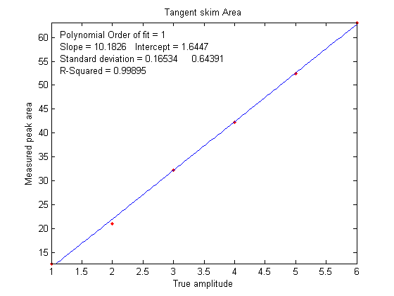
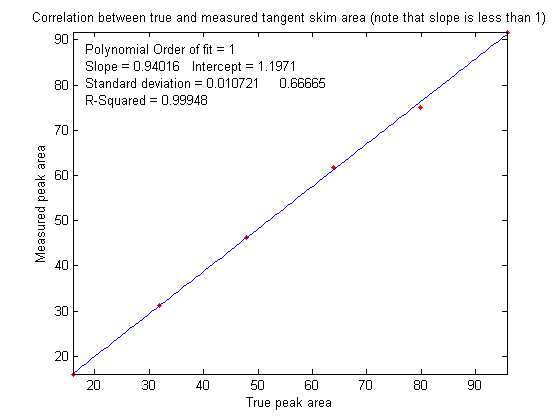
In this case, the tangent skim method works best, giving a
linear calibration curve (shown on the left) with the
highest R2.
In this type of application, the peak heights and/or area
measurements do not actually have to be accurate,
but they must be precise.
That's because the objective of an analytical method such as
flow injection or chromatography is not
to measure peak heights
and areas,
but rather to measure concentrations,
which is why calibration curves are used. Figure
6 shows the correlation between the measured tangent
skim areas and the actual true areas under the peaks in the
signal shown above, right; the slope of this plot shows that
the tangent skim areas are actually about 6% lower that the
true areas, but that does not make a difference in this case
because the standards and the unknown samples are measured
the same way. In some other
application, you may
actually need to measure the peak heights and/or areas
accurately, in which case curve fitting is generally the
best way to go.
If the peaks partly overlap, the measured peak heights and
areas may be effected. To reduce the problem, it may be
possible to reduce the overlap by using peak
sharpening methods, for example the derivative
method, deconvolution or the power transform method, as
demonstrated by the self-contained Matlab/Octave function PowerTransformCalibrationCurve.m.
Curve fitting the signal
data. Ordinary in curve fitting, such as the classical
least squares (CLS) method and in iterative
nonlinear least-squares, the selection of a model
shape is very important. But in quantitative analysis applications of curve
fitting, where the peak height or area measured by curve
fitting is used only to determine the concentration of
the substance that created the peak by constructing a calibration curve, having the exact
model shape is surprisingly uncritical. The Matlab/Octave script PeakShapeAnalyticalCurve.m shows that, for a single isolated peak whose shape is
constant and independent of concentration, if the wrong
model shape is used, the peak heights measured by curve fitting
will be inaccurate, but that error will be exactly the same for the unknown samples and
the known calibration standards, so the error will
"cancel out" and the measured concentrations will still
be accurate, provided you use the same inaccurate model for both
the known standards and the unknown samples. 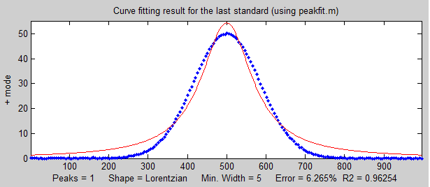 In
the
example shown on the right, the peak shape of the actual
peak is Gaussian (blue dots) but the model used to fit
the data is Lorentzian (red line). That's an intentionally
bad fit to the signal data; the R2 value for the
fit to the signal data is only 0.962 (a poor fit by the
standards of measurement science). The result of this is
that the slope of the calibration curve
(shown below on the left) is greater than expected; it should have been 10 (because that's the
value of the "sensitivity" in line 18), but it's
actually 10.867 in the figure on the left
In
the
example shown on the right, the peak shape of the actual
peak is Gaussian (blue dots) but the model used to fit
the data is Lorentzian (red line). That's an intentionally
bad fit to the signal data; the R2 value for the
fit to the signal data is only 0.962 (a poor fit by the
standards of measurement science). The result of this is
that the slope of the calibration curve
(shown below on the left) is greater than expected; it should have been 10 (because that's the
value of the "sensitivity" in line 18), but it's
actually 10.867 in the figure on the left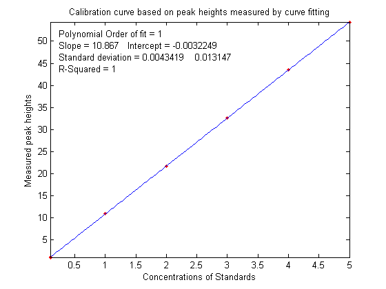 ,
but nevertheless the calibration curve is still
linear and its R2 value is 1.000,
meaning that the analysis should be accurate. (Note that
curve fitting is actually applied twice
in this type of
application, once using iterative curve fitting to fit
the signal data, and then again using polynomial curve fitting
to fit the calibration data).
,
but nevertheless the calibration curve is still
linear and its R2 value is 1.000,
meaning that the analysis should be accurate. (Note that
curve fitting is actually applied twice
in this type of
application, once using iterative curve fitting to fit
the signal data, and then again using polynomial curve fitting
to fit the calibration data).
Despite all this, it's still better to use as
accurate a model peak shape as possible for the signal
data, because the percent fitting error of the signal fit can be used as a warning that something
unexpected is wrong, such as the appearance of an
interfering peak from a foreign substance.