


Appendix AG. Using real-signal modeling to determine measurement
accuracy
It's common to use
computer-generated signals whose characteristics are known
exactly to establish the accuracy of a proposed signal
processing method, analogous to the use of standards in
analytical chemistry.
But the problem with computer-generated signals is that they are
often too simple or too ideal, such as a series of peaks that
are all equal in height and width, of some idealized shape such
as a pure Gaussian, and with idealized added random white noise.
For the measurement
of the areas of partly overlapping peaks, such ideal peaks will result in overly
optimistic estimates of area measurement accuracy. One way to
create more realistic known signals for a particular application
is to use iterative
curve fitting. If it is possible to find a model that fits the experimental
data very well, with very low fitting error and with random
residuals, then the peak parameters from that fit are used to
construct a more realistic synthetic signal that yield a much
better evaluation of the measurement. Moreover, synthetic
signals can be modified at will to explore how the proposed
measurement method might work under other experimental
conditions (e.g., if the sampling frequency were higher).
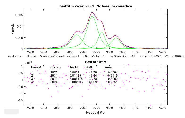 To
demonstrate this idea, I downloaded a spectrum from the NIST IR
database that contained a set of four highly fused peaks.
To determine the true peak areas as accurately as possible, I
iteratively fit those peaks with four GLS peaks (41% Gaussian)
of different widths, yielding a fitting error of only 0.3%, and
an R2 of 0.99988, with unstructured random residuals, as shown
on the left. The best-fit peak parameters and the residual noise
were then used in a self-contained script to create a synthetic
model signal that is essentially identical to the experimental
spectrum, except that it has exactly known peak areas. Then, the
script uses the simpler and faster perpendicular drop method to
measure those areas, using second differentiation to
locate the original peak positions, peak area measurement by perpendicular
drop, which by itself is not expected to work on such
overlapped peaks, and finally repeating the area measurements
after sharpening the peaks by Fourier
self-deconvolution, using a low-pass Fourier
filter to control the noise).
To
demonstrate this idea, I downloaded a spectrum from the NIST IR
database that contained a set of four highly fused peaks.
To determine the true peak areas as accurately as possible, I
iteratively fit those peaks with four GLS peaks (41% Gaussian)
of different widths, yielding a fitting error of only 0.3%, and
an R2 of 0.99988, with unstructured random residuals, as shown
on the left. The best-fit peak parameters and the residual noise
were then used in a self-contained script to create a synthetic
model signal that is essentially identical to the experimental
spectrum, except that it has exactly known peak areas. Then, the
script uses the simpler and faster perpendicular drop method to
measure those areas, using second differentiation to
locate the original peak positions, peak area measurement by perpendicular
drop, which by itself is not expected to work on such
overlapped peaks, and finally repeating the area measurements
after sharpening the peaks by Fourier
self-deconvolution, using a low-pass Fourier
filter to control the noise).
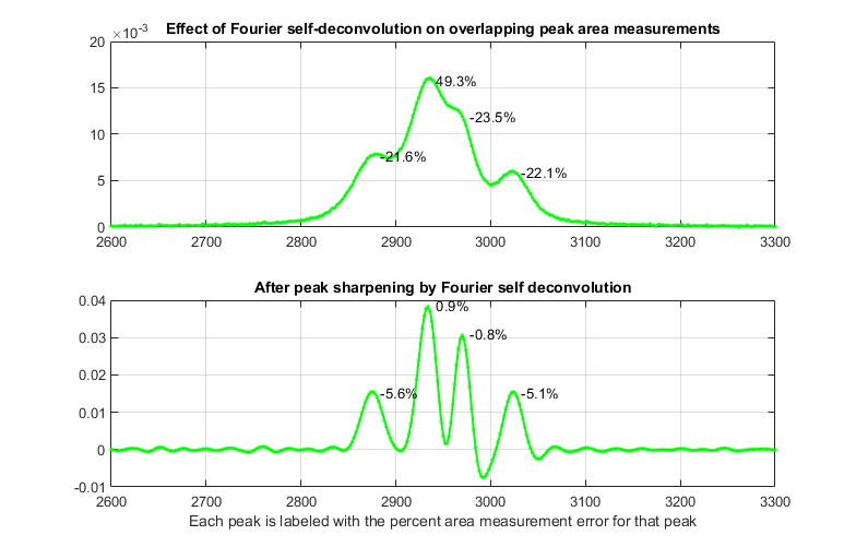
As shown by the first
figure below, self-deconvolution sharpening can in fact improve
the peak area accuracy substantially, from an average error of
29% for the original signal to only 3.1% after deconvolution.
But because the peaks have different widths, there is no single
optimum deconvolution width. Tests show that the best overall
results are obtained when the deconvolution function shape
is the same as in the original signal and when the deconvolution
function width is 1.1 times the average peak
width in the signal. In the second figure, the peaks in the
model signal have been spread out artificially, with no other
change, just to show more clearly that this choice of
deconvolution function width causes the third peak to be "over
sharpened", resulting in negative lobes for that peak. (But
recall that deconvolution is done in a way that conserves total
peak area). A more
conservative approach, using the largest deconvolution width possible without the
signal ever going negative (about 0.8 times the average peak width in this case) results in
only a modest improvement in area accuracy (from 27% to 12%; graphic).
Sampling interval (cm-1)= 2
Change in peak separation (PeakSpread)=
0
Noise= 5e-05
GLS Shape (fraction Gaussian)= 0.41
Deconvolution Width= 23.7 points
(1.1 times the mean signal peak width)
Frequency Cutoff= 20%
\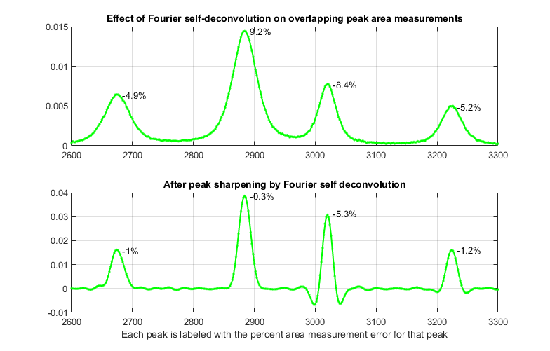
Change in peak separation
("PeakSpread") = 100. All other parameters are unchanged.
This
page is part of "A Pragmatic Introduction to Signal
Processing", created and maintained by Prof. Tom O'Haver ,
Department of Chemistry and Biochemistry, The University of
Maryland at College Park. Comments, suggestions and questions
should be directed to Prof. O'Haver at toh@umd.edu. Updated January, 2023.
